Multiclass Logistic Regression: One-vs-One, One-vs-All, and Softmax Explained

A concise guide to Multiclass Logistic Regression: extending logistic regression for multiclass problems. This article, "Multiclass Logistic Regression: One-vs-One, One-vs-All, and Softmax Explained," compares one-vs-all, one-vs-one, and softmax approaches with practical examples.

Introduction

In many machine learning tasks, we are interested in predicting a categorical outcome.
Binary Logistic Regression is one of the simplest and most fundamental models for such tasks — particularly designed for two-class (binary) problems.

Examples:

• Email spam detection
• Disease diagnosis (sick vs. healthy)
• Sentiment analysis (positive vs. negative)

However, real-world problems often involve more than two categories. For example:

• Classifying emails into spam, personal, or work
• Predicting the species of a flower from multiple types

In such scenarios, we extend logistic regression to multiclass classification.

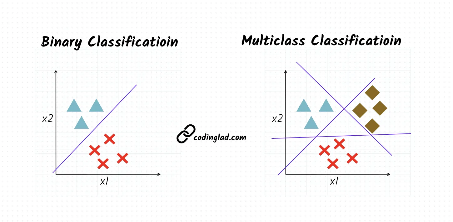
Extending Logistic Regression to Multiclass Classification

We extend logistic regression to handle multiple classes using these two key strategies:

🧠 One-vs-One (OvO)

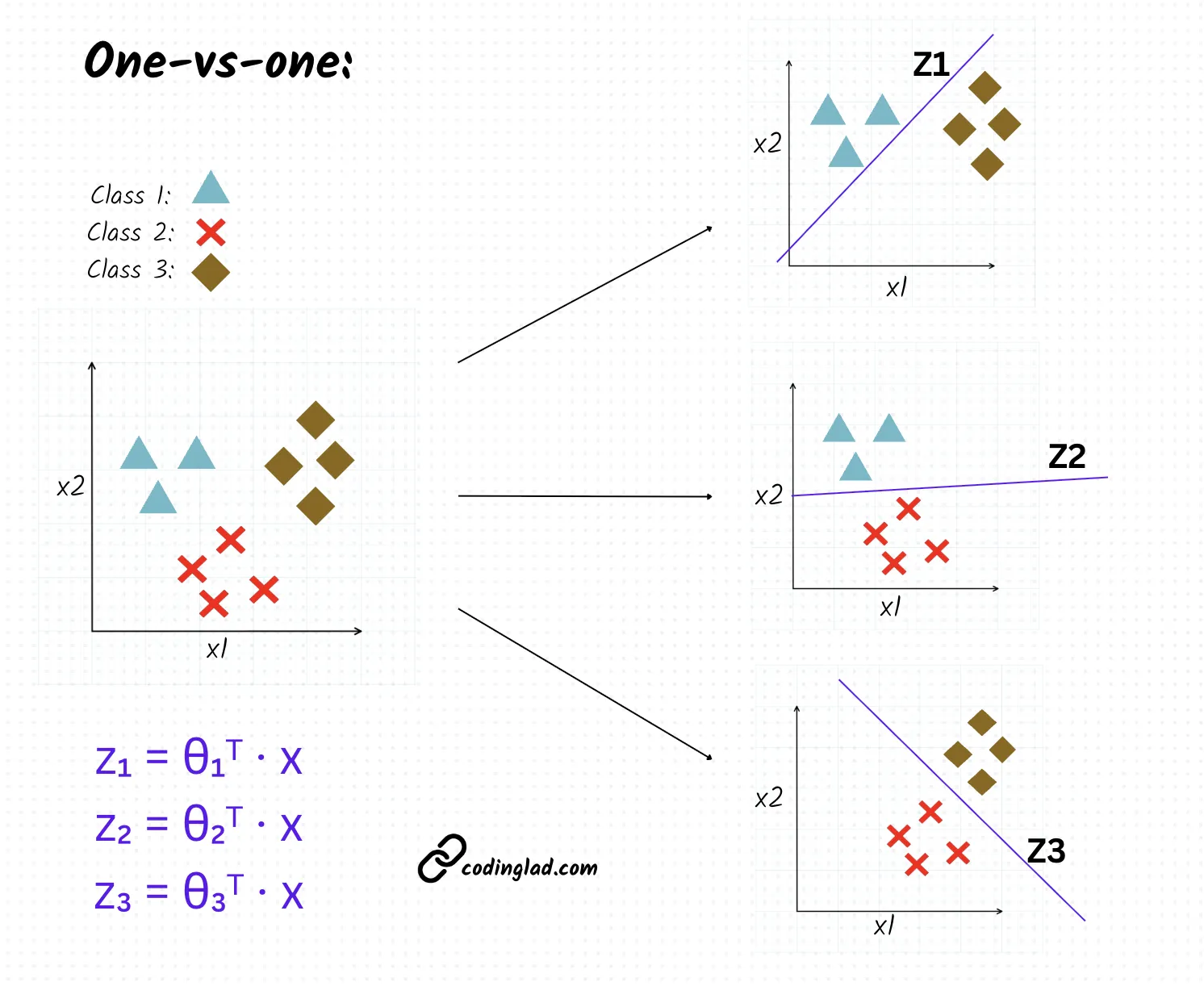
Strategy: Train $\frac{K(K-1)}{2}$ binary classifiers for $K$ classes - one for each pair.

Mechanics:

• Each classifier uses sigmoid to produce probabilities:

$$h_{\theta^{(i,j)}}(x) = \frac{1}{1 + e^{-\theta^{(i,j)\top}x}}$$

• Prediction threshold: If $h_{\theta^{(i,j)}}(x) > 0.5$, class $i$ gets a vote; else class $j$

🔢 Example Calculation (3 classes):

Classifiers	Probabilities	Votes
Class 1 vs 2	$h_{\theta^{(1,2)}}(x) = 0.7$	Class 1
Class 1 vs 3	$h_{\theta^{(1,3)}}(x) = 0.6$	Class 1
Class 2 vs 3	$h_{\theta^{(2,3)}}(x) = 0.6$	Class 2

Final Prediction: Class 1 (2 vote), Class 2 (1), Class 3 (0) → Class 1 wins!

🌐 One-vs-All (OvA)

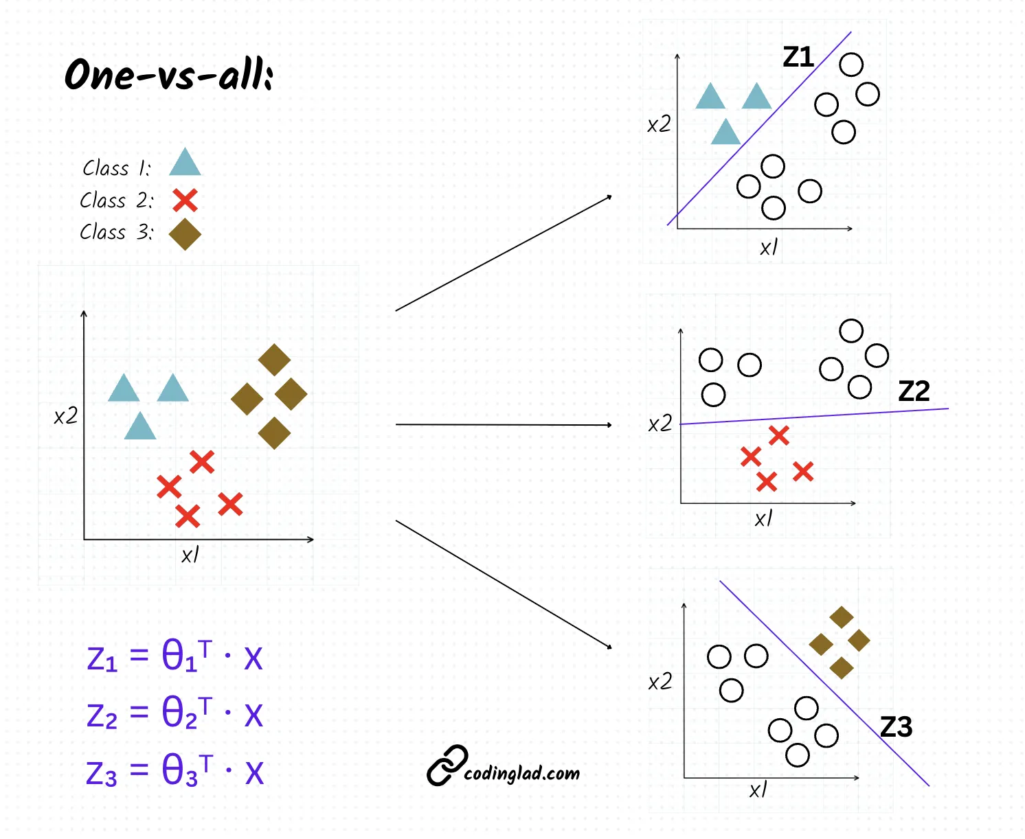
Strategy: Train $K$ classifiers - each distinguishes one class from all others.

Mechanics:

• Each classifier uses sigmoid for class probability:

$$h_{\theta^{(i)}}(x) = \frac{1}{1 + e^{-\theta^{(i)\top}x}}$$

• Final prediction: Class with highest probability score

🔢 Example Calculation (3 classes):

Classifier	Probability
Class 1 vs Rest	$h_{\theta^{(1)}}(x) = 0.85$
Class 2 vs Rest	$h_{\theta^{(2)}}(x) = 0.55$
Class 3 vs Rest	$h_{\theta^{(3)}}(x) = 0.25$

Final Prediction: Class 1 (max probability 0.85)

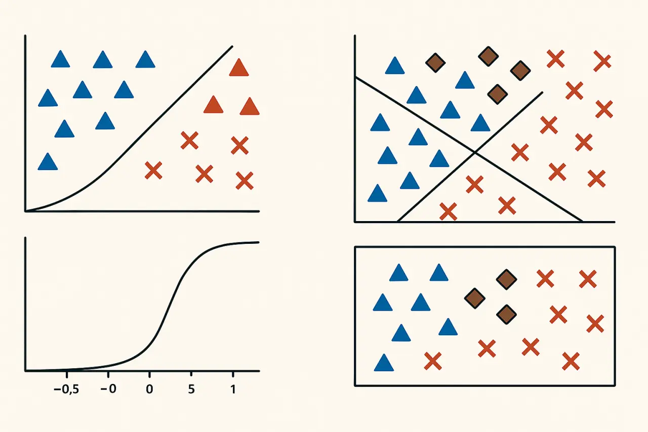
📈 Sigmoid Function: The Probability Engine

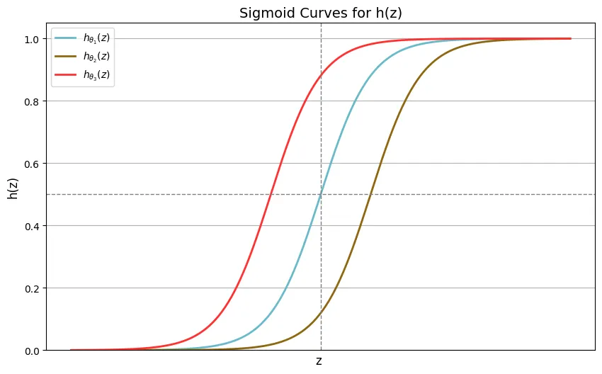
Both strategies rely on the sigmoid function to convert linear combinations into probabilities:

$$h_\theta(z) = \frac{1}{1 + e^{-z}} \quad \text{where } z = \theta^\top x$$

Key Properties:

• Squashes values between 0 and 1
• $z = 0$ gives $h = 0.5$ (decision boundary)
• Threshold at 0.5 for binary decisions
• Smooth gradient for optimization

🏆 Strategy Comparison

Feature	One-vs-One	One-vs-All
# Classifiers	$K(K-1)/2$ (Explosive growth)	$K$ (Linear growth)
Training Data Per Model	Balanced pairs	Imbalanced (1 vs many)
Best For	Small $K$, balanced classes	Large $K$, imbalanced data
Computation	More parallelizable	Less resource-intensive

🔥 Multinomial Logistic Regression (Softmax)

While OvO and OvA work by combining binary classifiers, they have a fundamental limitation: their probability scores don't form a proper probability distribution across all classes.

❌ The Probability Sum Problem

Consider our OvA example with 3 classes:

Classifier	Probability
Class 1 vs Rest	0.85
Class 2 vs Rest	0.55
Class 3 vs Rest	0.25

Total "probability": 0.85 + 0.55 + 0.25 = 1.65
(Not a valid probability distribution - should sum to 1)

This happens because each classifier operates independently without considering other classes' scores.

🎯 Softmax Solution

Multinomial Logistic Regression solves this using the softmax function to ensure probabilities are:

• Between 0 and 1
• Sum to 1 across all classes

Softmax Formula:

$$P(y=i|x) = \frac{e^{\theta_i^\top x}}{\sum_{j=1}^K e^{\theta_j^\top x}}$$

🔢 Example Calculation (3 classes):

Given raw scores (logits):

• Class 1: $z_1 = \theta_1^\top x = 2.0$
• Class 2: $z_2 = \theta_2^\top x = 1.0$
• Class 3: $z_3 = \theta_3^\top x = -1.0$

1. Compute exponents:

   • $e^{2.0} ≈ 7.389$
   • $e^{1.0} ≈ 2.718$
   • $e^{-1.0} ≈ 0.368$

2. Sum exponents:
   $7.389 + 2.718 + 0.368 ≈ 10.475$

3. Normalize:

   • $P(y=1) = 7.389/10.475 ≈ 0.705$
   • $P(y=2) = 2.718/10.475 ≈ 0.259$
   • $P(y=3) = 0.368/10.475 ≈ 0.035$

Total Probability: 0.705 + 0.259 + 0.035 = 1.0 ✅

🆚 Softmax vs Sigmoid Strategies

Feature	OvO/OvA + Sigmoid	Multinomial + Softmax
Probability Guarantee	No sum-to-1 constraint	Valid probability distribution
Class Interdependence	Treats classes independently	Models class relationships
Computation	Multiple binary models	Single unified model
Decision Boundary	Piecewise linear	Smooth global boundary
Scalability	Better for small K	More efficient for large K

💡 Key Insight: Softmax creates competition between classes - increasing one class' probability automatically decreases others' probabilities. This mimics how real-world categories often relate to each other.

⚙️ Shared Machinery: Cost, Learning & Evaluation

While multiclass strategies differ in their modeling approaches, they share common components in optimization and evaluation:

📉 Cost Functions

1. OvO & OvA (Binary Cross-Entropy)
Each binary classifier uses:

$$J(\theta) = -\frac{1}{m} \sum_{i=1}^m \left[y^{(i)} \log(h_\theta(x^{(i)})) + (1-y^{(i)}) \log(1-h_\theta(x^{(i)}))\right]$$

2. Softmax (Categorical Cross-Entropy)

Single unified cost function:

$$J(\theta) = -\frac{1}{m} \sum_{i=1}^{m} \sum_{k=1}^{K} y_k^{(i)} \log \left( \hat{y}_k^{(i)} \right)$$

Where:

• $y_k^{(i)}$ is 1 only for the correct class.
• $\hat{y}_k^{(i)}$ is the predicted probability for class $k$, computed via softmax.

Interpretation:

• $y_k^{(i)}$ is 1 if example $i$ belongs to class $k$, and 0 otherwise.
• $\hat{y}^k = P(y = k \mid x^{(i)}; \theta)$ is the predicted probability that example $i$ belongs to class $k$ under the current model parameters.

Softmax ensures the outputs are valid class probabilities that sum to 1

$$\hat{y}_k = \frac{e^{z_k}}{\sum_{j=1}^K e^{z_j}}$$

🧠 Learning: Gradient Descent Variations

Method	Parameters Updated	Computational Complexity
OvO	$\frac{K(K-1)}{2}$ independent θs	High (Requires training $\mathcal{O}(K^2)$ models)
OvA	$K$ independent θs	Moderate (K separate models)
Softmax	Single $K \times d$ parameter matrix	Efficient (Single model)

Example: Softmax Gradient Derivation
For class $j$ parameters $\theta_j$:

$$\nabla_{\theta_j} J(\Theta) = \frac{1}{m} \sum_{i=1}^m x^{(i)}\left(p_j^{(i)} - y_j^{(i)}\right)$$

Where:

• $p_j^{(i)} = P(y^{(i)} = j|x^{(i)})$ (softmax probability)
• $y_j^{(i)} = \mathbb{I}[\text{True class} = j]$ (indicator function)

Update Rule for Softmax:

$$\theta_j := \theta_j - \alpha \nabla_{\theta_j} J(\Theta)$$ $$\Rightarrow \theta_j := \theta_j - \frac{\alpha}{m} \sum_{i=1}^m x^{(i)}\left(p_j^{(i)} - y_j^{(i)}\right)$$

Key Differences:

1. OvO/OvA: Requires parallel gradient updates across multiple independent models
2. Softmax: Single coherent update across all classes using matrix operations
3. Numerical Stability: Softmax implementations typically use log-sum-exp trick

📊 Evaluation: Cross-Validation & Metrics

Common Practices Across All Methods:

1. Basic Train/Test Split

• Split the dataset into two parts: a training set (e.g., 80%) and a test set (e.g., 20%).
• Train the model on the training set.
• Evaluate performance (accuracy, precision, recall, F1-score, etc.) on the test set.
• Simple and fast, but results can vary depending on how the data is split.

2. k-Fold Cross-Validation

• Divide the dataset into k equal-sized folds (e.g., k=5 or 10).
• For each fold:
  • Use that fold as the validation set, and the remaining k-1 folds as the training set.
  • Train and evaluate the model.
• Average the results across all k runs for a more robust estimate of model performance.
• OvO/OvA require refitting all pairwise/one-vs-rest models per fold.
• Helps reduce variance due to random data splits and gives a better sense of generalization.

🔄 End-to-End Process Comparison

Step	OvO/OvA	Softmax
1. Training	Train multiple binary models	Train single multiclass model
2. Prediction	Aggregate votes/scores	Direct probability computation
3. Cross-Validation	Validate each model separately	Validate unified model
4. Hyperparameter Tuning	Tune each model or global params	Single parameter space tuning

Practical Tip: Use class LogisticRegression(multi_class='multinomial') in sklearn to access softmax implementation directly. For OvO/OvA, use OneVsOneClassifier or OneVsRestClassifier wrappers.

🏁 When to Use Which?

• Binary Classification: Sigmoid (logistic regression)
• Small K, Fast Prototyping: OvO/OvA
• Theoretical Correctness: Softmax
• Large-Scale Production: Softmax
• Class Imbalance: Softmax (handles relative probabilities better)