Time & Space Complexity — Notes

Time & Space Complexity — Notes
These notes explain how to measure an algorithm’s cost as the input gets bigger.
Two things to keep in mind while reading:
- When we say a line of code takes “1 unit of time,” we mean one basic step—not a real clock second. The goal is to see how the work grows with input size, not to predict exact runtime.
- For space, we usually count only extra memory the algorithm creates (like temporary variables or arrays)—not the original input itself.
1. What is Complexity?
Two major criteria are used to analyze an algorithm:
- Time Complexity → How the running time grows as the input size grows.
- Space Complexity → How much extra memory the algorithm needs as the input size grows.
We usually represent input size with n.
Basic idea
For analysis, we can think of:
- 1 basic operation ≈ 1 unit of time
- 1 variable ≈ 1 unit of space
These are simplified models used to understand how an algorithm scales.
EXAMPLE 1 — Swap Function
def swap(a, b):
    temp = a
    a = b
b = tempTime Complexity
temp = a    → 1 step
a = b       → 1 step
b = temp → 1 stepTotal:
f(n) = 33 is a constant and does not depend on the input size.
Think of f(n) as a simple polynomial in n. Here there is no n term, so the degree is 0:
f(n) = 3          → degree 0
O(3) → O(1)Degree tip: For polynomials like , Big-O is usually , where is the degree. Constant → degree 0 → .
Space Complexity
Only one extra variable is created:
tempSo:
Space = O(1)Key idea
If the amount of work/memory stays constant regardless of input size → O(1).
EXAMPLE 2 — Single Loop
def print_all(arr):
    for i in arr:
print(i)Assume arr contains n elements.
Time Complexity
The loop runs n times:
print(i) → 1 step × nTherefore:
f(n) = nThis is a polynomial of degree 1 (the highest power of n is ):
f(n) = n          → degree 1
Time = O(n)Space Complexity
No extra data structure grows with n.
The loop variable i uses constant space.
Space = O(1)Note: The input array itself is not counted as extra/auxiliary space.
Key idea
One loop that processes every element → usually O(n).
EXAMPLE 3 — Nested Loops
def print_pairs(arr):
    for i in arr:
        for j in arr:
print(i, j)Assume arr has n elements.
Time Complexity
Outer loop:
n timesFor each outer iteration, the inner loop runs:
n timesTherefore:
n × n = n²f(n) = n²Highest power of n is , so degree 2:
f(n) = n²         → degree 2
Time = O(n²)Rule
Nested loops → multiply their work. Degree usually matches how many times
nis multiplied.
n × n       → degree 2 → O(n²)
n × n × n → degree 3 → O(n³)For example:
for i in arr:          # n
    for j in arr:      # n
        for k in arr:  # n
...Time = O(n³)EXAMPLE 4 — Input Gets Cut in Half
Binary Search
def binary_search(arr, target):
    low, high = 0, len(arr) - 1

    while low <= high:
        mid = (low + high) // 2

        if arr[mid] == target:
            return mid
        elif arr[mid] < target:
            low = mid + 1
        else:
high = mid - 1The important idea is that after each iteration, roughly half of the remaining elements are eliminated.
n
↓
n/2
↓
n/4
↓
n/8
↓
...
↓
1We ask:
How many times can we divide
nby 2 before reaching 1?
That is:
log₂(n)Therefore:
Time = O(log n)Rule
If the problem size is repeatedly divided by a constant factor → O(log n).
Examples:
n → n/2 → n/4 → n/8 → ...This is different from simply removing one element:
n → n-1 → n-2 → n-3 → ...The second pattern is usually O(n).
EXAMPLE 5 — Divide + Combine
Merge Sort
def merge_sort(arr):
    if len(arr) <= 1:
        return arr

    mid = len(arr) // 2

    left = merge_sort(arr[:mid])   # divide left half
    right = merge_sort(arr[mid:])  # divide right half

    return merge(left, right)      # combine sorted halves


def merge(left, right):
    """Merge two already-sorted lists into one sorted list."""
    result = []
    i = j = 0

    while i < len(left) and j < len(right):
        if left[i] <= right[j]:
            result.append(left[i])
            i += 1
        else:
            result.append(right[j])
            j += 1

    result.extend(left[i:])
    result.extend(right[j:])
return resultHow merge compares elements matters:
It does not compare the whole left half against one right element.
Both halves are already sorted, so we only compare the current fronts with two pointers i and j:
compare left[i] vs right[j]
  → take the smaller one
→ move that pointer forward by 1Each comparison advances exactly one element into result. After at most about len(left) + len(right) takes, both halves are used up.
Example:
left  = [3, 27, 38, 43]
right = [9, 10, 56, 82]

3 vs 9  → take 3
27 vs 9 → take 9
27 vs 10 → take 10
27 vs 56 → take 27
... and so onSo work is linear in the combined size, not “left size × right size”.
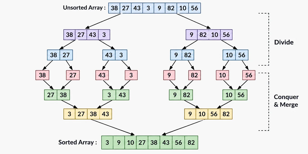
Merge sort has two parts — divide the array, then merge sorted halves back together:
Part 1 — Divide
The array is repeatedly divided in half:
n
n/2
n/4
n/8
...
1Number of levels:
log nPart 2 — Combine
Each call to merge(left, right) walks through both halves once:
left  has about n/2 elements  → up to n/2 steps
right has about n/2 elements  → up to n/2 steps
───────────────────────────────────────────────
one merge → about n/2 + n/2 = n stepsSo merging one pair of halves is for that subproblem size.
Across a whole level of the tree, every element is merged exactly once, so the total work per level is still:
O(n)Therefore:
O(n) per level × O(log n) levelsTime = O(n log n)Space Complexity
Merge sort typically needs extra arrays/storage for merging.
The total auxiliary space is:
Space = O(n)Key idea
Divide into halves + linear work at each level → O(n log n).
EXAMPLE 6 — Recursion That Branches
Naive Fibonacci
def fib(n):
    if n <= 1:
        return n

return fib(n - 1) + fib(n - 2)Each call makes two more recursive calls:
fib(n)
├── fib(n-1)
│   ├── fib(n-2)
│   └── fib(n-3)
└── fib(n-2)
    ├── fib(n-3)
└── fib(n-4)The number of calls grows exponentially.
A simplified model is:
2^nTherefore:
Time = O(2^n)Space Complexity
The recursion does not create all calls simultaneously.
The deepest chain is approximately:
n → n-1 → n-2 → ... → 1So the maximum call-stack depth is n.
Space = O(n)Important
Time and space are calculated separately.
Time  = O(2^n)
Space = O(n)QUICK RULES
1. Sequential operations → ADD
If operations happen one after another:
O(1) + O(n)Keep the dominant term:
O(n)Example:
do_constant_work()   # O(1)

for x in arr:        # O(n)
...Total:
O(1) + O(n) = O(n)2. Nested operations → MULTIPLY
If one operation runs inside another:
O(n) × O(n)Then:
O(n²)Example:
for i in arr:
    for j in arr:
...→ O(n²)
3. Drop Constants
Constants don't matter for Big-O growth.
O(2n)   → O(n)
O(500)  → O(1)
O(10n²) → O(n²)4. Drop Smaller Terms
Keep the term that grows fastest — for polynomials, that is the highest degree.
O(n² + n) → O(n²)          → degree 2 wins

O(n³ + n² + n) → O(n³)     → degree 3 wins

O(n + 100) → O(n) → degree 1 winsdegree 0 → O(1)
degree 1 → O(n)
degree 2 → O(n²)
degree 3 → O(n³)This degree shortcut is for polynomial growth. Logs (), , exponentials (), and factorials () are different patterns.
5. Different Inputs → Keep Them Separate
Suppose:
for x in A:
    ...

for y in B:
...If:
A has a elements
B has b elementsThen:
Time = O(a + b)NOT:
O(n)unless you know that a and b are both represented by the same n.
Similarly:
for x in A:
    for y in B:
...gives:
O(a × b)ORDER OF GROWTH
From better / slower-growing to worse / faster-growing:
O(1)
  ↓
O(log n)
  ↓
O(n)
  ↓
O(n log n)
  ↓
O(n²)
  ↓
O(2ⁿ)
  ↓
O(n!)Growth Rate Comparison
As grows, faster curves pull away — that’s why Big-O matters more than “it works on my laptop.”
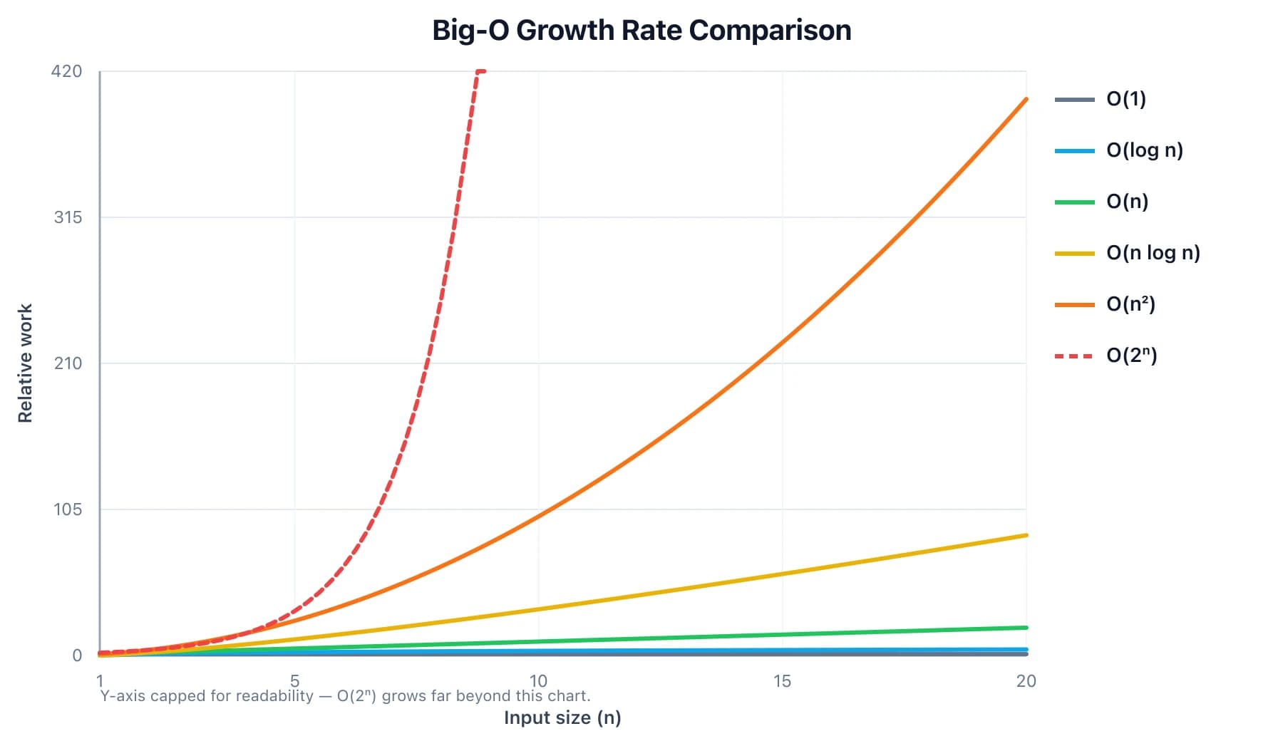
How to read it: and stay nearly flat. and rise steadily. bends up hard. shoots off the chart almost immediately — so the Y-axis is capped for readability.
Common Examples
| Complexity | Example |
|---|---|
| O(1) | Swap two variables |
| O(log n) | Binary search |
| O(n) | Print all elements |
| O(n log n) | Merge sort |
| O(n²) | Print all pairs, bubble sort |
| O(2ⁿ) | Naive Fibonacci |
| O(n!) | Generate all permutations |
The Patterns to Remember
Instead of memorizing every algorithm, recognize these patterns:
Constant work
        ↓
     O(1)


Input processed once
        ↓
     O(n)


Input repeatedly halved
        ↓
    O(log n)


Two full nested loops
        ↓
    O(n²)


Divide into halves + process everything at each level
        ↓
   O(n log n)


Two recursive branches at every level
        ↓
    O(2ⁿ)


Try every possible ordering
        ↓
O(n!)One-line mental model
ADD for sequential work, MULTIPLY for nested work, LOG when the input is repeatedly divided, and analyze TIME and SPACE separately.