How Neural Networks Use GPUs Differently — Compute, Memory & Parallelism

Table Of Content
- 1. What Are We Comparing?
- 2. Five Architectures from a GPU Perspective
- DLRM — Recommendation Models
- MLP — Dense Neural Network
- Weight reuse example — house prices
- CNN — Convolutional Neural Network
- MLP vs CNN — weight sharing
- RNN — Recurrent Neural Network
- Why RNNs exist — variable length and memory
- Word order matters
- Hidden state walkthrough — “I love AI”
- The key equation difference
- Parallelism comparison — MLP vs CNN vs RNN
- Transformer
- Self-attention example — “The cat sat on the mat”
- Simplified attention score matrix
- RNN sequential vs Transformer parallel
- Why long sequences get expensive
- KV cache during generation
- 3. The Central Comparison
- 4. Compute-Bound vs Memory-Bound
- 5. Why Discuss These Five Together?
- 6. Test Your Understanding
- Final Takeaway
- Q&A — Conceptual, Math & Comparison
How Neural Networks Use GPUs Differently — Compute, Memory & Parallelism
Not every neural network puts the same kind of pressure on a GPU.
Some models spend most of their time calculating. Others spend most of their time waiting for data. Some can run huge amounts of work in parallel. Others are stuck waiting for the previous step to finish.
This post looks at five common architectures — DLRM, MLP, CNN, RNN, and Transformer — through that GPU lens.
Central idea: memorize three dimensions — computation, memory movement, and parallelism — then see how each architecture behaves differently along those dimensions.
1. What Are We Comparing?
Three questions sit behind the whole comparison:
- Compute-bound or memory-bound? Does the model spend more time performing calculations, or waiting for data from memory?
- Parallelism: Can the GPU perform many operations at once, or must it wait for previous operations?
- Memory access and reuse: Does the model repeatedly reuse the same data, or does it keep fetching different data from memory?
Those three ideas explain most of the differences between these workloads.
2. Five Architectures from a GPU Perspective
DLRM — Recommendation Models
Imagine you’re using YouTube.
YouTube needs to decide which video to recommend next.
It has information about:
- You (user ID)
- The video (item ID)
- Your watch history
- Video category
- Your previous interactions
- Other numerical information about your activity
DLRM (Deep Learning Recommendation Model) combines these different types of information to predict a score.
For example:
The model estimates how likely you are to click a particular video.
▸What is DLRM? (short overview)
DLRM (Deep Learning Recommendation Model) is used for ranking and recommendation systems — for example, which ads or products to show a user.
It combines:
- Sparse categorical features (user ID, item ID) looked up from large embedding tables
- Dense features processed by an MLP
- A final MLP that predicts a score (click, conversion, etc.)
The distinctive GPU challenge is not the MLP part — it is the irregular embedding lookups into huge tables.
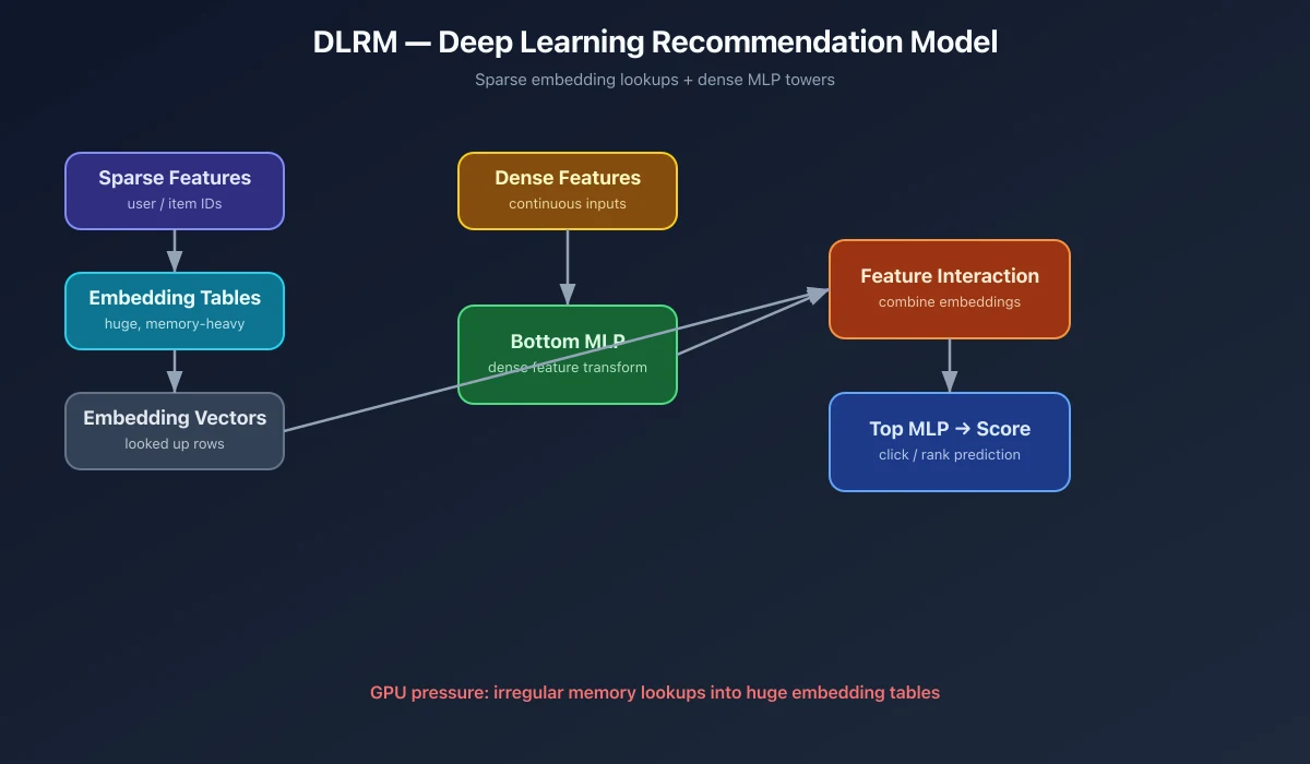
Tendency: memory-bound
Imagine a recommendation model with 100 million user embeddings.
When a user asks for a recommendation, the GPU needs to fetch specific embedding vectors from memory.
- Lots of data needs to be stored.
- Memory locations accessed are often unpredictable.
- Relatively little computation happens per lookup.
- Data movement becomes expensive.
GPU challenge: fetching data efficiently matters more than raw calculation speed.
For a concrete implementation example, see NVIDIA’s DLRM for PyTorch.
MLP — Dense Neural Network
Imagine an email app deciding whether a message is spam.
The app converts the email into a list of numbers — for example word counts, sender reputation, time of day, and other features.
Those numbers are fed into stacked fully connected layers:
- Every input connects to every neuron in the next layer
- Each layer transforms the representation
- The final layer outputs a probability
For example:
That dense, fully connected structure is an MLP.
▸What is an MLP? (short overview)
An MLP (Multilayer Perceptron) is a classic fully connected neural network: stacked layers where every neuron connects to every neuron in the next layer.
Each layer is basically a matrix multiply:
That maps extremely well onto GPUs, especially with large batch sizes that reuse the same weights across many samples.
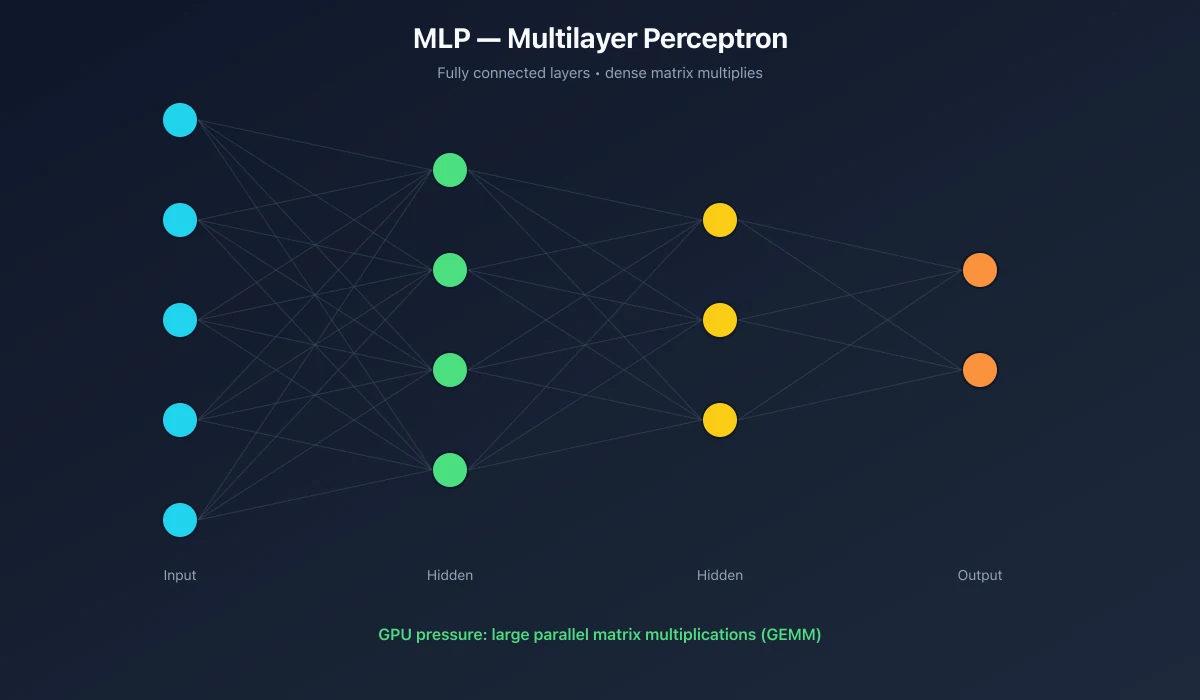
Tendency: compute-intensive, often compute-bound
In a multilayer perceptron, every input connects to every output through weights.
The GPU performs large matrix multiplications.
- Many multiplication and addition operations.
- Same weights reused across multiple samples.
- Matrix operations can be executed in parallel.
GPU advantage: GPUs are especially good at matrix multiplication.
Large batches improve weight reuse and can make computation the dominant cost.
Weight reuse example — house prices
Let’s say we’re building an MLP to predict house prices for 3 houses.
Each house has two input features:
- House size
- Number of bedrooms
We want to produce one output: predicted house price.
Each row represents a different house.
Suppose the trained MLP has these weights:
These weights are shared across all three houses.
Look at this:
House 1
- Input:
- Same
- Uses weights and
House 2
- Input:
- Same
- Uses weights and again
House 3
- Input:
- Same
- Uses weights and again
Notice that we don’t need a separate weight matrix for each house.
The GPU loads the weight matrix once and uses it to process multiple input rows.
That’s weight reuse.
Imagine processing 1,000 houses:
- The same weight matrix is used 1,000 times.
- Instead of loading completely different weights for every house, the GPU can reuse the same weights.
- Multiple houses can be processed simultaneously through matrix multiplication.
This means more computation can be performed for each time the weights are loaded from memory.
CNN — Convolutional Neural Network
Imagine you open Google Photos and search for “dog.”
The app looks at a photo pixel by pixel, but not by connecting every pixel to every weight. Instead, small filters slide across the image and detect patterns:
- Edges and textures in early layers
- Eyes, fur, and shapes in deeper layers
- “This looks like a dog” at the end
For example:
That sliding-filter approach is a CNN.
▸What is a CNN? (short overview)
A CNN (Convolutional Neural Network) is built for grid-like data such as images.
Instead of connecting every pixel to every weight, a small filter (kernel) slides across the image and detects local patterns — edges, textures, shapes.
Key idea: weight sharing — the same filter is reused across all spatial locations, which cuts parameters and improves data reuse on the GPU.
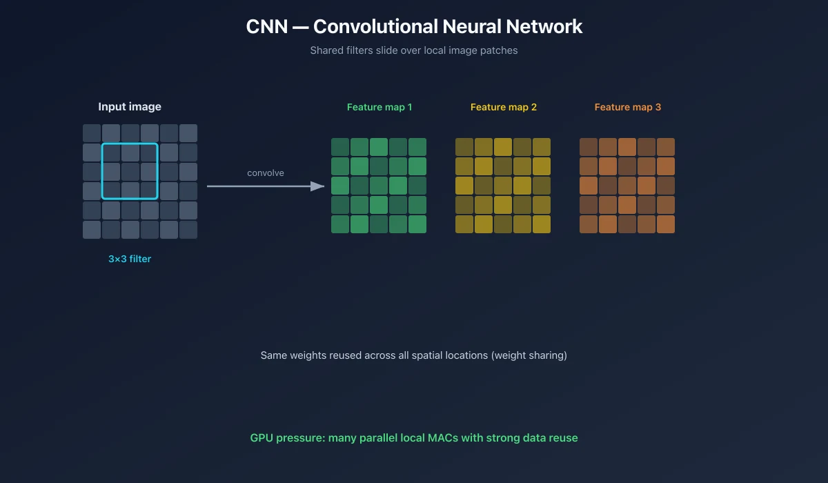
Tendency: compute-intensive, often compute-bound
The same small filter moves across different image regions.
- Same weights reused many times.
- Different image locations can be processed in parallel.
- Lots of multiplication and addition operations.
GPU advantage: weight sharing and local data reuse make convolution efficient.
However, small or depthwise convolutions can become memory-bound or overhead-bound.
MLP vs CNN — weight sharing
Let’s compare MLP and CNN.
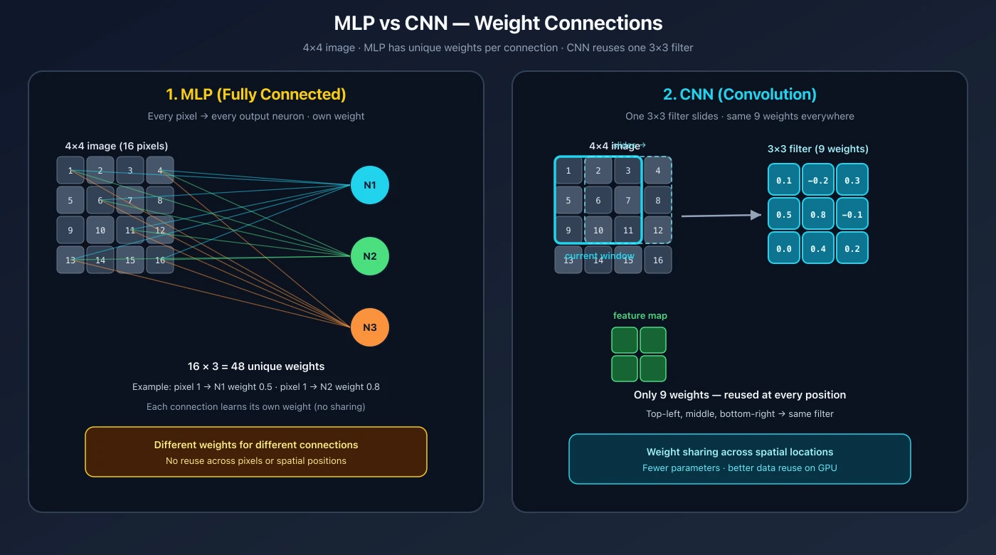
1. In a fully connected network (MLP)
Imagine a 4×4 image containing 16 pixels.
If we connect those 16 pixels to 3 output neurons, every pixel connects to every output neuron.
That means:
- weights
- Each connection has its own weight
For example, pixel 1 might have weight for neuron 1, but weight for neuron 2.
2. In a CNN
Instead of connecting every pixel to every output neuron, a CNN uses a small filter, such as a 3×3 kernel.
For a short CNN introduction, see
DataCamp’s CNN overview
.
The filter contains only 9 weights.
It examines a small region of the image, calculates an output, then moves to another region.
Here’s the important part: the same 9 weights are reused at every position.
The CNN doesn’t learn a completely new set of 9 weights for every image region.
3. Why is this useful?
Imagine detecting a vertical edge.
You want to detect that edge whether it appears:
- At the top-left corner
- In the middle
- At the bottom-right corner
The same filter can detect it in all three locations.
So:
- MLP: different weights for different input-output connections
- CNN: same filter weights reused across different spatial locations
That’s what we mean by weight sharing in CNNs. It reduces the number of parameters and allows efficient reuse of data and computations.
RNN — Recurrent Neural Network
Imagine an old-style phone keyboard predicting the next word as you type.
You type:
I love machineThe model reads one word at a time and keeps a memory of what came before:
- After “I” → memory updates
- After “love” → memory updates again
- After “machine” → it predicts the next word
For example:
Because each step depends on the previous hidden state, an RNN must process the sequence in order.
▸What is an RNN? (short overview)
An RNN (Recurrent Neural Network) processes sequences step by step — text, audio, time series.
At each time , it updates a hidden state using the current input and the previous hidden state :
That recurrence is why RNNs struggle to parallelize across time: step must wait for step .
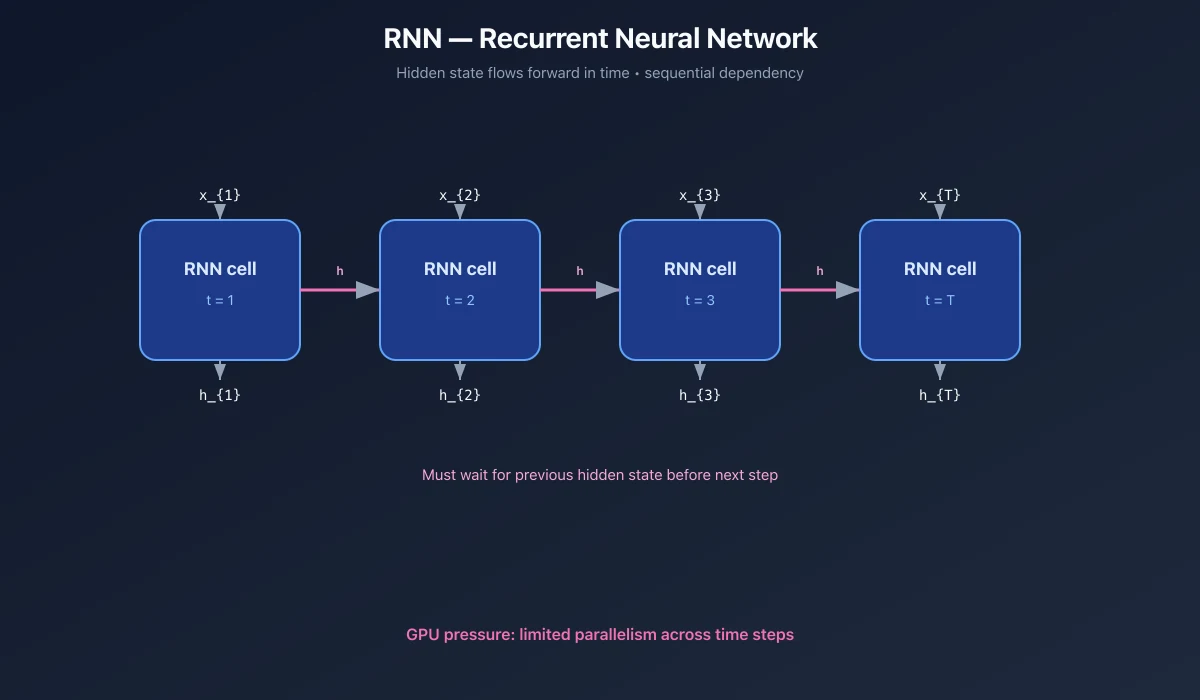
Tendency: sequential dependency
An RNN processes a sequence one time step at a time.
- The next step needs the previous hidden state.
- The GPU cannot freely execute all time steps simultaneously.
- More GPU compute units cannot remove this dependency.
GPU challenge: limited parallelism across the sequence.
RNNs can still perform parallel computation across batch elements and within each time step. For a standard walkthrough of the recurrence, see CS231n on RNNs.
Why RNNs exist — variable length and memory
Imagine you’re building a neural network to process sentences.
Consider these two sentences:
- “I love AI”
- “I love learning artificial intelligence”
They have different numbers of words.
In a traditional feedforward neural network (MLP), the input layer has a fixed number of neurons.
For example, if you design an input layer with 3 neurons, it expects 3 input values.
What happens if the input contains 10 words instead?
RNN solves this by processing sequential inputs one at a time.
It can process 3 words, 10 words, or 100 words using the same network parameters.
Word order matters
Suppose we have two sentences:
- “Dog bites man”
- “Man bites dog”
Both contain exactly the same words, but their meanings are different because the order changes.
A traditional MLP doesn’t have a mechanism for remembering what it processed previously.
It receives its input features and processes them through its layers.
It can learn different weights for different input positions, so changing the order can change its output. But it doesn’t inherently maintain a sequential memory of previous inputs.
RNN introduces that memory through something called a hidden state.
Hidden state walkthrough — “I love AI”
An RNN processes the sentence one word at a time.
Input 1: “I”
- RNN processes the first word
- Produces hidden state
- is the memory of “I”
Input 2: “love”
- RNN processes both the current input and the previous hidden state
- Produces a new hidden state
- contains updated information
Input 3: “AI”
- RNN uses the current word and
- Produces
- carries information from previous steps
Notice what happens:
- First input produces hidden state
- Second input uses both the current word and to produce
- Third input uses the current word and to produce
This is the important difference: the previous output (hidden state) is reused when processing the next input.
The key equation difference
MLP
Only the current input is used.
RNN
Current input + previous hidden state are used.
That’s it. RNN adds the previous hidden state to the normal neural network equation, giving it memory of previous inputs — and that same dependency is why the GPU cannot freely parallelize across time steps.
Parallelism comparison — MLP vs CNN vs RNN
MLP — high parallelism
Multiple input samples can be processed simultaneously.
- Each sample can be processed independently using the same weights.
- Matrix multiplication allows thousands of operations to execute in parallel.
- The same weight matrix is reused across different samples in a batch.
CNN — high parallelism
Multiple image regions can be processed simultaneously using the same convolution filter.
- Instead of connecting every pixel to every output neuron, a CNN uses a small filter, such as a 3×3 kernel.
- The same filter slides across different image locations.
- This reduces the number of parameters and often the computation required compared with fully connected image processing.
- Different spatial positions and output channels can be calculated in parallel.
The key difference from MLP: CNN uses local connections and shared filters, while MLP uses fully connected layers.
RNN — limited parallelism across time
- First, calculate .
- Then calculate using .
- Then calculate using .
You cannot calculate all time steps independently because each step needs the previous hidden state.
The key difference: unlike MLP and CNN, an RNN has a sequential dependency between time steps.
| Model | Parallelism | Why |
|---|---|---|
| MLP | High | Independent samples × shared weights |
| CNN | High | Shared filter across spatial locations |
| RNN | Limited across time | depends on |
Transformer
Imagine ChatGPT answering your question.
Your prompt is split into tokens:
"Explain" "GPU" "memory"Unlike an RNN, a Transformer can look at all tokens together during training or encoding. Each token can attend to every other token — for example, relating “memory” back to “GPU.”
When generating the reply, it still writes one token at a time, but it reuses previous Key/Value computations through a KV cache.
For example, after seeing the prompt, it may assign high attention between related words and then generate:
"GPU memory stores tensors..."That attention-based design is a Transformer.
▸What is a Transformer? (short overview)
A Transformer replaces recurrence with self-attention: every token can look at every other token in the sequence.
During training, that enables excellent parallelism across tokens. The tradeoff is cost — full attention scales about like in sequence length .
During generation, models often store a KV cache so previous keys/values are not recomputed, which grows GPU memory as the sequence gets longer.
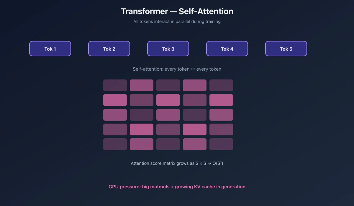
Tendency: highly parallel, attention- and memory-intensive
Unlike RNNs, Transformers can process all input tokens in parallel during training.
But every token can interact with every other token.
- Excellent parallelism during training.
- Attention computation grows quadratically with sequence length.
- The KV cache consumes increasing memory during generation.
GPU challenge: handling large attention computations and memory requirements.
Self-attention example — “The cat sat on the mat”
Let’s use a simple example: predicting the next word in the sentence “The cat sat on the mat.”
Imagine the Transformer receives these tokens:
| Token | Word |
|---|---|
| Token 1 | The |
| Token 2 | cat |
| Token 3 | sat |
| Token 4 | on |
| Token 5 | mat |
Each token is converted into a numerical representation called an embedding.
Every token looks at the other tokens to understand their relevance.
For example:
- “cat” pays attention to “sat” to understand what the cat is doing.
- “sat” pays attention to “cat” to understand who performed the action.
- “mat” pays attention to “on” to understand the relationship.
The model calculates attention scores between tokens.
Simplified attention score matrix
Illustrative values, not actual model outputs.
| The | cat | sat | on | mat | |
|---|---|---|---|---|---|
| The | 0.4 | 0.3 | 0.1 | 0.1 | 0.1 |
| cat | 0.1 | 0.3 | 0.4 | 0.1 | 0.1 |
| sat | 0.1 | 0.4 | 0.3 | 0.1 | 0.1 |
| on | 0.1 | 0.1 | 0.2 | 0.2 | 0.4 |
| mat | 0.1 | 0.1 | 0.2 | 0.2 | 0.4 |
Each row represents one token’s attention distribution across the sequence.
The important thing: these attention calculations can be performed in parallel during training. The model doesn’t need to finish processing “The” before processing “cat”.
RNN sequential vs Transformer parallel
Consider the same sentence.
RNN — sequential processing
The → h1
cat → h2
sat → h3
on  → h4
mat → h5The RNN must calculate the hidden state for “The” before “cat”, then “cat” before “sat”, and so on.
Transformer — parallel processing during training
The   cat   sat   on   mat
 ↓     ↓     ↓    ↓     ↓
all processed together via self-attentionAll token representations can be processed together through self-attention.
That’s why Transformers offer much better parallelism across sequence positions during training.
Why long sequences get expensive
Suppose a sentence has:
- 5 tokens → attention scores
- 100 tokens → scores
- 1,000 tokens → scores
So longer sequences create significantly more computation and memory pressure — attention grows like .
KV cache during generation
Now imagine the model generates a sentence one token at a time.
It has already processed:
"The cat sat"Now it needs to generate the next token.
Instead of recalculating the Key and Value representations for “The cat sat”, it stores them in GPU memory. This stored information is called the KV cache.
When it generates “on”, it adds the new token’s Key and Value to the cache. When it generates “the” next, it reuses the previous cache and adds the new ones.
KV cache growth
- After generating “The” → 1 token stored
- After generating “cat” → 2 tokens stored
- After generating “sat” → 3 tokens stored
- After generating “on” → 4 tokens stored
The cache keeps growing as the generated sequence gets longer.
Why this matters for GPUs: the KV cache occupies GPU memory. Longer conversations and longer generated sequences require more memory to store previous Keys and Values.
3. The Central Comparison
| Model | Main GPU challenge | Parallelism |
|---|---|---|
| DLRM | Memory access | Irregular lookups |
| MLP | Matrix computation / weight movement | Excellent |
| CNN | Repeated convolution | Excellent |
| RNN | Sequential dependency | Limited across time |
| Transformer | Attention computation / KV cache | Excellent during training |
Notice that there are two separate concepts:
- Compute-bound vs memory-bound describes what limits performance.
- Parallelism describes how much work can execute simultaneously.
They are related, but they are not the same thing.
4. Compute-Bound vs Memory-Bound
Compute-bound — waiting for calculations
The GPU already has enough data available, but it needs time to perform all the mathematical operations.
Adding more computational power can improve performance.
Example: a large matrix multiplication.
Memory-bound — waiting for data
The GPU could calculate faster, but it spends time waiting for data to arrive from memory.
Adding more computational units may not solve the problem.
Example: random embedding lookups in DLRM.
A kitchen analogy
Imagine a restaurant kitchen:
- Compute-bound: the kitchen has all the ingredients, but the chef needs time to cook.
- Memory-bound: the chef is fast, but ingredients are not arriving from the storage room quickly enough.
For more background on GPU parallelism, see Dive Into Systems — GPUs.
5. Why Discuss These Five Together?
Because different ML workloads need different hardware optimizations.
| If the workload is... | Hardware optimization that helps |
|---|---|
| DLRM | High memory capacity, bandwidth, efficient data access |
| MLP | Fast matrix multiplication, tensor cores |
| CNN | Convolution acceleration, data reuse |
| RNN | Faster sequential execution, optimized recurrent operations |
| Transformer | Fast matrix multiplication, attention acceleration, efficient KV cache |
This matters because a GPU designed mainly to accelerate matrix multiplication may perform exceptionally well on MLPs, yet still struggle with irregular embedding lookups or sequential RNN dependencies.
6. Test Your Understanding
Question 1
A recommendation model randomly fetches millions of embedding vectors. What is its main bottleneck?
- GPU calculation speed
- Memory access and data movement
- Sequential dependency
▸Show answer
Answer: Memory access and data movement. The compute per lookup is small; the hard part is fetching scattered embedding vectors.
Question 2
An RNN processes 100 tokens, where each step depends on the previous hidden state. What limits parallelism?
- Memory capacity
- Dense connectivity
- Sequential dependency
▸Show answer
Answer: Sequential dependency. Time step cannot start until time step finishes.
Question 3
A large MLP performs massive matrix multiplications using the same weights across many samples. Which hardware capability helps most?
- Parallel matrix computation
- Random memory lookup
- Sequential execution
▸Show answer
Answer: Parallel matrix computation. Dense layers map cleanly onto GPU matrix engines and tensor cores.
Question 4
Why can Transformer attention become expensive for long sequences?
- It cannot process tokens in parallel
- Every token can interact with every other token
- It uses no weight sharing
▸Show answer
Answer: Every token can interact with every other token, so attention cost grows with sequence length — roughly for standard attention — and KV cache grows during generation.
Final Takeaway
Do not memorize five architectures as five disconnected topics.
Memorize the three dimensions:
computation
memory movement
parallelismThen ask, for each model:
What is the GPU waiting on?
How much work can run at the same time?
How often is data reused vs freshly fetched?That is the real story: different neural networks stress GPU hardware differently, so the right optimization depends on the workload.
Q&A — Conceptual, Math & Comparison
Part A: Conceptual Questions
Q1. What is the difference between a compute-bound and a memory-bound workload?
▸Show answer
Answer:
A compute-bound workload spends most of its time performing mathematical operations. The GPU’s computational capacity is the primary performance limitation.
A memory-bound workload spends a significant amount of time waiting for data to arrive from memory. The GPU may have unused computational capacity because data is not being supplied quickly enough.
Examples:
- Compute-bound: large matrix multiplication.
- Memory-bound: random embedding lookups in DLRM.
Q2. Why is DLRM considered a memory-intensive workload?
▸Show answer
Answer:
DLRM uses large embedding tables containing millions or billions of entries. Each recommendation request retrieves only a small subset of these embeddings.
The problem is that these lookups often access unpredictable memory locations. Fetching scattered embedding vectors can become expensive, even when the actual computation per lookup is relatively small.
Therefore, DLRM is often limited by memory capacity and memory bandwidth rather than raw GPU computing power.
Q3. Why is MLP suitable for GPU parallelism?
▸Show answer
Answer:
MLP performs dense matrix multiplication, where multiple input samples and output features can be processed simultaneously.
GPUs are specifically designed to perform large numbers of multiplication and accumulation operations in parallel.
Additionally, the same weight matrix can be reused across multiple samples in a batch, improving data reuse and computational efficiency.
Q4. What is weight sharing in CNNs, and why is it important?
▸Show answer
Answer:
Weight sharing means using the same convolution filter across different spatial locations of an image.
For example, a filter designed to detect vertical edges can be reused across the entire image rather than learning separate weights for every location.
This reduces the number of parameters and allows the GPU to reuse filter weights across many computations.
Q5. Why are RNNs difficult to parallelize across time steps?
▸Show answer
Answer:
An RNN maintains a hidden state that carries information from one time step to the next.
The hidden state at time step depends on the previous hidden state at .
Therefore, the next time step cannot complete its computation until the previous state becomes available.
This sequential dependency limits parallelism across the sequence, even when the GPU has many available computing units.
Q6. Why can Transformers process tokens in parallel during training, unlike traditional RNNs?
▸Show answer
Answer:
Traditional RNNs require the previous hidden state before processing the next time step.
Transformers use self-attention, which computes relationships between tokens using matrix operations. During training, the input sequence can be processed together without waiting for the previous token’s hidden state.
This enables substantial parallelism across the sequence.
However, autoregressive generation still produces new tokens sequentially.
Q7. Why does Transformer attention become expensive for long sequences?
▸Show answer
Answer:
In standard full self-attention, every token can interact with every other token.
For a sequence of length , the attention score matrix contains approximately elements per attention head.
Therefore, doubling the sequence length increases the number of attention scores by approximately four times.
This is why long-context processing creates significant computational and memory demands.
Q8. What is KV cache, and why is it used in Transformers?
▸Show answer
Answer:
KV cache stores previously calculated Key and Value representations during autoregressive generation.
Without KV cache, the model would need to recompute the keys and values for previous tokens repeatedly when generating each new token.
By storing and reusing them, the model avoids unnecessary recomputation.
However, KV cache consumes additional GPU memory as the sequence grows.
Q9. What is the difference between parallelism and computational intensity?
▸Show answer
Answer:
Parallelism describes how much work can be executed simultaneously.
Computational intensity describes how much computation is performed relative to the amount of data transferred from memory.
A workload can have excellent parallelism but still be memory-bound if it requires too much data movement.
These are separate characteristics and should not be confused.
Part B: Mathematical Questions
Q10. Calculate the total embedding memory required by a DLRM model.
A recommendation model contains:
- Number of embedding entries: 100 million
- Embedding dimension: 128
- Data type: FP32 (4 bytes per value)
Calculate the total embedding table memory.
▸Show answer
Formula:
Solution:
Answer: 51.2 GB (approximately 47.7 GiB).
Q11. Calculate the embedding payload accessed in one DLRM batch.
Suppose:
- Batch size
- Average embedding rows retrieved per sample
- Embedding dimension
- FP32 values bytes
Calculate the total embedding data accessed.
▸Show answer
Formula:
Solution:
Answer: 1 MiB of embedding data.
Notice that the entire embedding table requires 51.2 GB, but this batch accesses only 1 MiB of embedding data.
Q12. Calculate MACs and FLOPs for an MLP layer.
An MLP has:
- Batch size
- Input features
- Output features
Calculate the total MACs and FLOPs.
▸Show answer
Formulas:
Solution:
Answer:
- MACs = 8.39 million
- FLOPs = 16.78 million
Q13. Calculate the weight memory required by an MLP layer.
Suppose an MLP has 1024 input features and 512 output features. Each weight uses FP32 (4 bytes).
▸Show answer
Formula:
Solution:
Answer: 2 MiB.
Q14. Calculate the number of MACs in a CNN convolution layer.
Given:
- Batch size
- Output height
- Output width
- Kernel size
- Input channels
- Output channels
Calculate the total MACs.
▸Show answer
Formula:
Solution:
Answer: 4.72 million MACs.
Q15. Calculate the approximate MACs of a vanilla RNN.
Given:
- Batch size
- Sequence length
- Input dimension
- Hidden dimension
Calculate the approximate number of MACs.
▸Show answer
Formula:
Solution:
Answer: 78.64 million MACs.
Q16. How does Transformer attention complexity change when sequence length doubles?
Suppose a Transformer processes 1,000 tokens. Its sequence length increases to 2,000 tokens.
▸Show answer
Standard full attention scales as:
For 1,000 tokens:
For 2,000 tokens:
Answer: The number of attention scores increases by 4 times.
This demonstrates why long sequences create significant attention-related computational and memory costs.
Q17. Calculate the KV cache memory required by a Transformer.
Suppose:
- Batch size
- Sequence length
- Model dimension
- FP16 data type (2 bytes per value)
Calculate the KV cache memory per layer using standard multi-head attention.
▸Show answer
Formula:
The first factor of 2 represents Key and Value storage.
Solution:
Answer: Approximately 3.91 MiB per layer.
Part C: Analytical and Comparison Questions
Q18. Compare the five architectures in terms of their primary GPU bottlenecks.
▸Show answer
| Architecture | Primary characteristic |
|---|---|
| DLRM | Memory capacity, bandwidth, and irregular access |
| MLP | Dense computation and weight movement |
| CNN | Repeated convolution and weight reuse |
| RNN | Sequential dependency across time steps |
| Transformer | Attention computation and KV cache memory |
Note that these are typical workload tendencies, not absolute classifications. Actual performance depends on batch size, model dimensions, implementation, and hardware.
Q19. What happens when batch size increases in an MLP?
▸Show answer
Answer:
Increasing batch size increases the amount of computation and activation memory.
However, the weight matrix remains the same size and can be reused across more samples.
This improves weight reuse and can increase computational efficiency, potentially making the workload more compute-bound.
Q20. Can adding more GPU cores completely solve the sequential dependency problem in RNNs?
▸Show answer
Answer:
No. More GPU cores can accelerate calculations within individual time steps and process different batch elements simultaneously.
However, the dependency between consecutive time steps remains. The next hidden state still requires the previous hidden state.
Therefore, adding more computing units cannot completely eliminate the sequential critical path.
Q21. Which architecture benefits most from weight sharing, and why?
▸Show answer
Answer:
CNNs benefit significantly from weight sharing.
The same convolution filters are reused across different image locations, reducing the number of parameters and allowing efficient reuse of weights during computation.
Q22. Why might a GPU perform well on MLP workloads but struggle with DLRM workloads?
▸Show answer
Answer:
MLPs primarily perform dense matrix multiplication, which maps efficiently to GPU parallel computing units and tensor cores.
DLRMs rely heavily on embedding lookups that access unpredictable memory locations.
Therefore, a GPU with excellent matrix multiplication performance may still experience bottlenecks when handling irregular memory access and large embedding tables.
Final Revision: Formulas to Remember
| Architecture | Formula | What it calculates |
|---|---|---|
| DLRM | Total embedding memory | |
| DLRM | Embedding payload per batch | |
| MLP | MACs | |
| MLP | FLOPs | |
| MLP | Weight memory | |
| CNN | MACs | |
| RNN | MACs | |
| Transformer | Attention computation scaling | |
| Transformer | KV cache memory per layer |