Graphs in Python — Beginner-Friendly Notes

Table Of Content
- 1. What Is a Graph?
- 2. Basic Graph Terminology
- 3. Undirected Graphs
- 4. Directed Graphs
- 5. Weighted Graphs
- 6. How Do We Store a Graph?
- 7. Adjacency List
- 8. Adjacency Matrix
- 9. Adding Vertices and Edges
- 10. What Is Graph Traversal?
- 11. Breadth-First Search (BFS)
- 12. Depth-First Search (DFS)
- 13. BFS vs DFS
- 14. Finding a Path with BFS
- 15. Disconnected Graphs
- 16. Why Do We Need visited?
- 17. Graph vs Tree
- 18. Common Graph Mistakes
- 19. Complexity Summary
- Quick Rules
- Final Summary
Graphs in Python — Beginner-Friendly Notes
A graph represents relationships between different objects.
For example:
People       → friendships
Cities       → roads
Web pages    → links
Computers    → network connections
Courses → prerequisitesGraphs are useful whenever the relationship between objects is as important as the objects themselves.
1. What Is a Graph?
A graph consists of two main parts:
- Vertices — the objects
- Edges — the connections between those objects
A vertex is also called a node.
Consider this graph:
A ─── B
│     │
│     │
C ─── DThe vertices are:
A, B, C, DThe edges are:
A — B
A — C
B — D
C — DWe can write the graph mathematically as:
G = (V, E)where:
V = set of vertices
E = set of edgesFor this graph:
V = {A, B, C, D}
E = {(A, B), (A, C), (B, D), (C, D)}A graph is a collection of vertices connected by edges.
2. Basic Graph Terminology
Consider:
A ─── B ─── D
│
│
CAdjacent vertices
Two vertices are adjacent if an edge directly connects them.
A and B are adjacent.
A and C are adjacent.
A and D are not adjacent.Neighbor
A vertex directly connected to another vertex is its neighbor.
Neighbors of A = B, C
Neighbors of B = A, DDegree
The degree of a vertex is the number of edges connected to it.
degree(A) = 2
degree(B) = 2
degree(C) = 1
degree(D) = 1Path
A path is a sequence of vertices connected by edges.
C → A → B → Dis a path from C to D.
Path length
In an unweighted graph, path length is the number of edges in the path.
C → A → B → Dcontains three edges, so its length is 3.
Cycle
A cycle is a path that returns to its starting vertex.
A → B → D → C → AConnected graph
An undirected graph is connected if every vertex can be reached from every other vertex.
3. Undirected Graphs
In an undirected graph, an edge works in both directions.
A ─── BThis means:
A is connected to B
B is connected to AExamples:
- Facebook friendship
- Two-way roads
- Computers connected through a local network
If (A, B) is an undirected edge, then (B, A) represents the same connection.
4. Directed Graphs
In a directed graph, every edge has a direction.
A → BThis means A points to B, but B does not necessarily point to A.
Examples:
- Instagram following
- Web-page links
- Course prerequisites
- One-way roads
A → Band:
B → Aare different directed edges.
In-degree and out-degree
In a directed graph:
- In-degree = number of edges coming into a vertex
- Out-degree = number of edges leaving a vertex
A → B → C
    ↑
DFor B:
in-degree(B)  = 2   # from A and D
out-degree(B) = 1 # toward C5. Weighted Graphs
A weighted graph assigns a value called a weight to every edge.
       5
A ───────── B
│           │
│ 2         │ 3
│           │
C ───────── D
4Weights may represent:
- Distance
- Travel time
- Cost
- Network delay
- Difficulty
For example:
A → B has weight 5
A → C has weight 2In an unweighted graph, we usually treat every edge as having the same cost.
6. How Do We Store a Graph?
A diagram helps humans understand a graph, but a program needs a data structure.
The two most common representations are:
- Adjacency list
- Adjacency matrix
Consider:
A ─── B
│     │
│     │
C ─── D7. Adjacency List
An adjacency list stores the neighbors of every vertex.
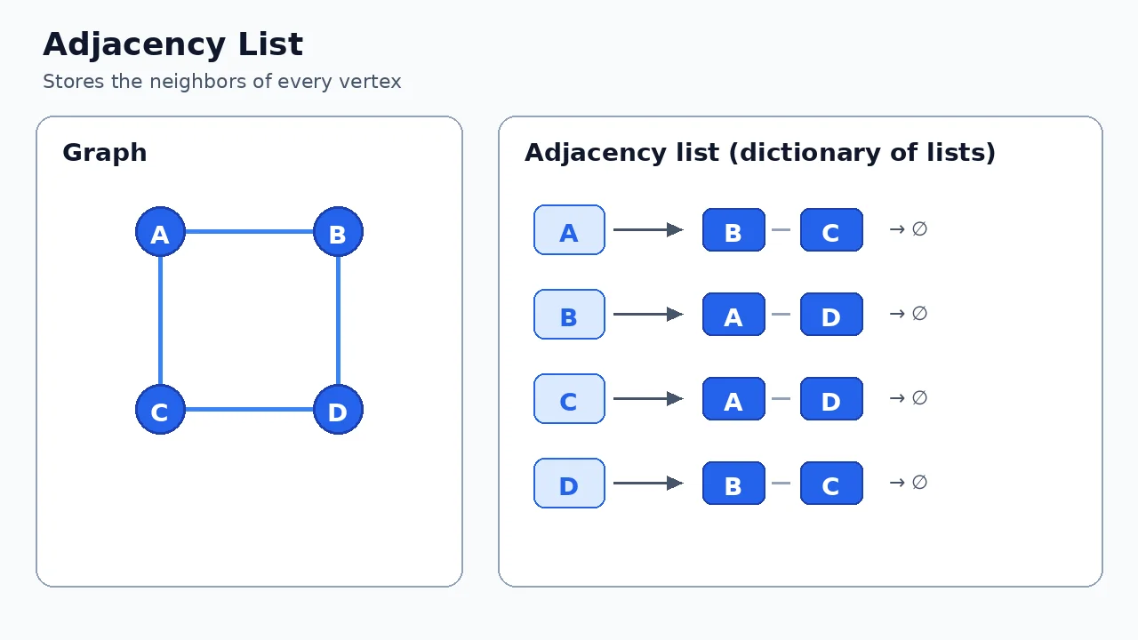
In Python, an adjacency list is usually a dictionary:
- each key is a vertex
- each value is a list of that vertex’s neighbors
graph = {
    "A": ["B", "C"],
    "B": ["A", "D"],
    "C": ["A", "D"],
    "D": ["B", "C"]
}For example:
print(graph["A"])Output:
['B', 'C']Because the graph is undirected, every connection appears in both vertices' lists:
A contains B
B contains ADirected adjacency list
For:
A → B
A → C
B → Dwe store only outgoing neighbors:
graph = {
    "A": ["B", "C"],
    "B": ["D"],
    "C": [],
    "D": []
}Weighted adjacency list
For a weighted graph, store both the neighbor and weight:
graph = {
    "A": [("B", 5), ("C", 2)],
    "B": [("A", 5), ("D", 3)],
    "C": [("A", 2), ("D", 4)],
    "D": [("B", 3), ("C", 4)]
}Space complexity
If a graph has V vertices and E edges:
Space = O(V + E)Adjacency lists are especially efficient for sparse graphs, where relatively few edges exist.
8. Adjacency Matrix
An adjacency matrix uses a two-dimensional grid.
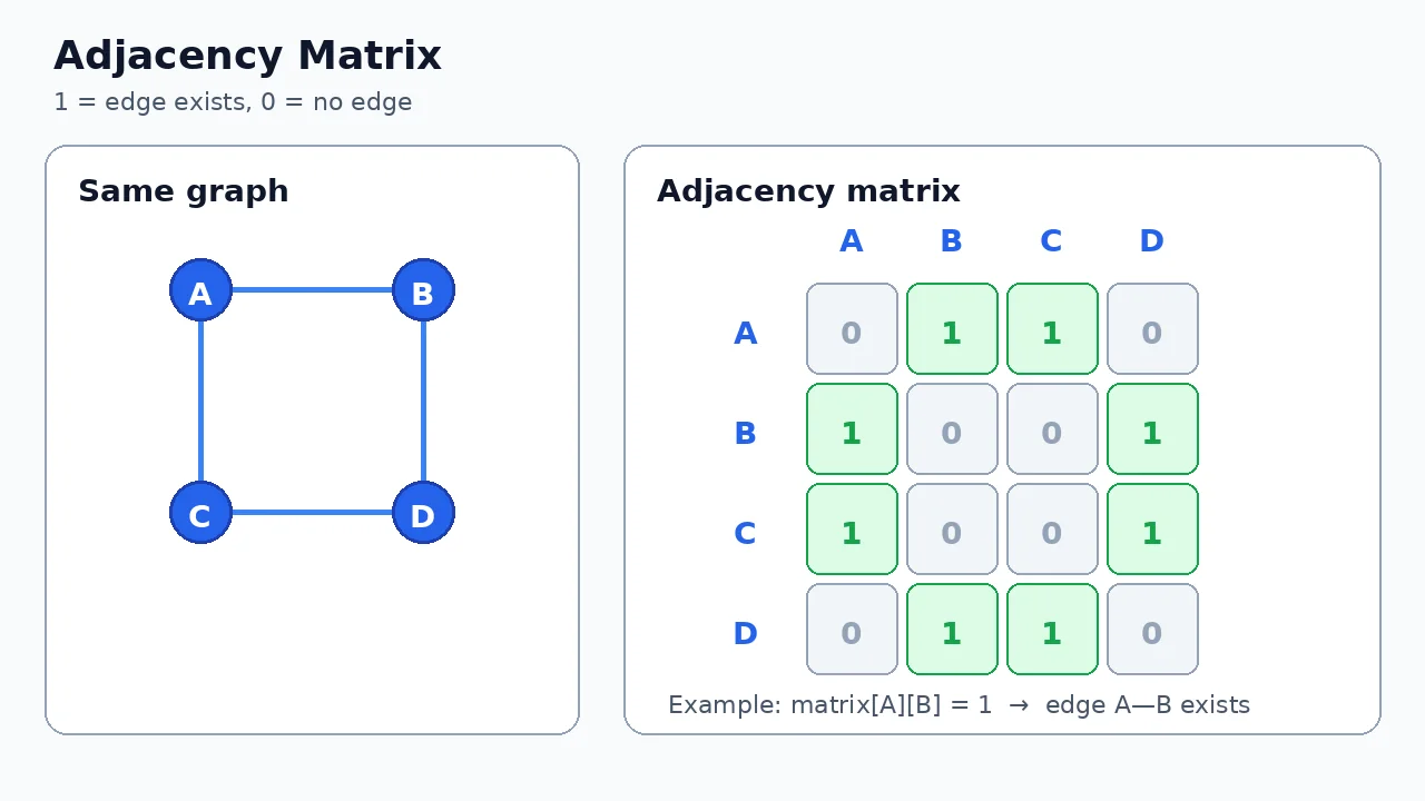
    A  B  C  D
A [ 0, 1, 1, 0 ]
B [ 1, 0, 0, 1 ]
C [ 1, 0, 0, 1 ]
D [ 0, 1, 1, 0 ]Here:
1 → an edge exists
0 → no edge existsIn Python, an adjacency matrix is usually a 2D list (a list of lists):
- rows and columns follow the same vertex order, such as
A, B, C, D matrix[i][j] == 1means an edge exists between those two vertices
#    A  B  C  D
matrix = [
    [0, 1, 1, 0],  # A
    [1, 0, 0, 1],  # B
    [1, 0, 0, 1],  # C
    [0, 1, 1, 0],  # D
]Because this graph is undirected, the matrix is symmetric: if matrix[A][B] = 1, then matrix[B][A] = 1 as well.
Directed adjacency matrix
For a directed graph, rows are sources and columns are destinations.
A → B
A → C
B → D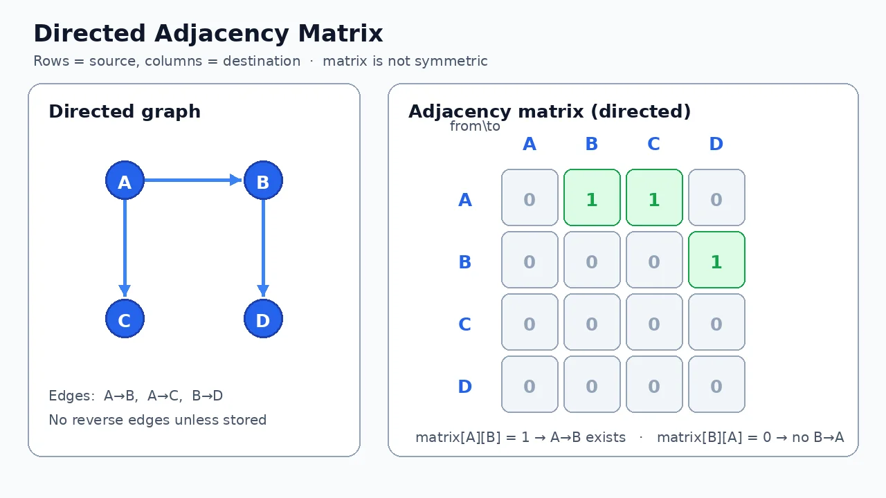
    A  B  C  D
A [ 0, 1, 1, 0 ]
B [ 0, 0, 0, 1 ]
C [ 0, 0, 0, 0 ]
D [ 0, 0, 0, 0 ]Python representation:
#    A  B  C  D
matrix = [
    [0, 1, 1, 0],  # A → B, A → C
    [0, 0, 0, 1],  # B → D
    [0, 0, 0, 0],  # C has no outgoing edges
    [0, 0, 0, 0],  # D has no outgoing edges
]Now the matrix is not symmetric:
matrix[A][B] = 1   → A → B exists
matrix[B][A] = 0 → B → A does not existChecking whether an edge exists is fast:
matrix[0][1] # A is connected to BTime = O(1)However, a matrix reserves space for every possible pair of vertices:
Space = O(V²)Adjacency list vs matrix
| Feature | Adjacency list | Adjacency matrix |
|---|---|---|
| Space | O(V + E) | O(V²) |
| Check a specific edge | Up to O(degree) | O(1) |
| Visit all neighbors | Efficient | Must scan a row |
| Best for | Sparse graphs | Dense graphs |
Most graph algorithms use adjacency lists because real-world graphs are often sparse.
9. Adding Vertices and Edges
We can build an undirected graph using a dictionary of lists:
graph = {}


def add_vertex(graph, vertex):
    if vertex not in graph:
        graph[vertex] = []


def add_edge(graph, first, second):
    add_vertex(graph, first)
    add_vertex(graph, second)

    graph[first].append(second)
graph[second].append(first)Using it:
add_edge(graph, "A", "B")
add_edge(graph, "A", "C")
add_edge(graph, "B", "D")Result:
{
    "A": ["B", "C"],
    "B": ["A", "D"],
    "C": ["A"],
    "D": ["B"]
}For a directed graph, add the edge only once:
def add_directed_edge(graph, source, destination):
    if source not in graph:
        graph[source] = []

    if destination not in graph:
        graph[destination] = []

graph[source].append(destination)10. What Is Graph Traversal?
Graph traversal means systematically visiting vertices in a graph.
Unlike an array, a graph does not always have one obvious starting point or direction.
The two main traversal algorithms are:
- Breadth-First Search (BFS)
- Depth-First Search (DFS)
Both need a visited set so that the same vertex is not processed repeatedly.
Consider:
        A
       / \
      B   C
     / \   \
D E F11. Breadth-First Search (BFS)
BFS explores the graph level by level.
Starting from A:
Level 0: A
Level 1: B, C
Level 2: D, E, FTraversal order:
A, B, C, D, E, FBFS uses a queue:
First In, First Out (FIFO)In Python, we usually implement this with collections.deque.
A deque (double-ended queue) is a generalized queue that allows insert and delete at both ends:
front ←→ back
  popleft() / appendleft()      pop() / append()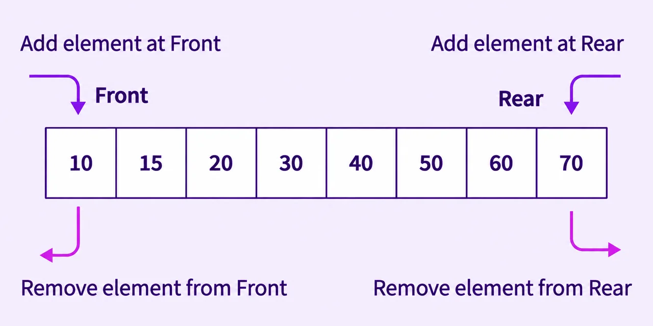
For BFS, we only need one side for each operation:
append(neighbor)  → add at the back
popleft() → remove from the frontThat keeps FIFO order and makes both operations .
BFS implementation
from collections import deque


def bfs(graph, start):
    visited = {start}
    queue = deque([start])

    while queue:
        vertex = queue.popleft()
        print(vertex)

        for neighbor in graph[vertex]:
            if neighbor not in visited:
                visited.add(neighbor)
queue.append(neighbor)Graph:
graph = {
    "A": ["B", "C"],
    "B": ["A", "D", "E"],
    "C": ["A", "F"],
    "D": ["B"],
    "E": ["B"],
    "F": ["C"]
}Calling:
bfs(graph, "A")Output:
A
B
C
D
E
FStep-by-step queue state
Queue [A]       → visit A → add B, C
Queue [B, C]    → visit B → add D, E
Queue [C, D, E] → visit C → add F
Queue [D, E, F] → visit D
Queue [E, F]    → visit E
Queue [F]       → visit F
Queue [] → finishedWhy mark a vertex when adding it?
We add a vertex to visited when it enters the queue:
visited.add(neighbor)
queue.append(neighbor)If we wait until removing it, multiple vertices may add the same neighbor to the queue.
BFS complexity
With an adjacency list:
Time  = O(V + E)
Space = O(V)Each vertex is visited once, and each edge is examined a limited number of times.
When BFS is useful
- Finding the shortest path in an unweighted graph
- Finding people within a certain number of social connections
- Level-order exploration
- Finding connected components
- Checking reachability
12. Depth-First Search (DFS)
DFS follows one path as deeply as possible before returning and trying another path.
For the same graph, one possible DFS order is:
A, B, D, E, C, FThe exact order depends on how neighbors are stored.
DFS can use:
- Recursion and the call stack
- An explicit stack
Recursive DFS
def dfs(graph, vertex, visited=None):
    if visited is None:
        visited = set()

    visited.add(vertex)
    print(vertex)

    for neighbor in graph[vertex]:
        if neighbor not in visited:
dfs(graph, neighbor, visited)Calling:
dfs(graph, "A")One possible output:
A
B
D
E
C
FExecution idea:
A
└── B
    └── D
        └── no unvisited neighbor → return
    └── E
        └── no unvisited neighbor → return
└── C
└── FThe recursive calls use the call stack automatically.
Iterative DFS
def dfs_iterative(graph, start):
    visited = set()
    stack = [start]

    while stack:
        vertex = stack.pop()

        if vertex in visited:
            continue

        visited.add(vertex)
        print(vertex)

        for neighbor in reversed(graph[vertex]):
            if neighbor not in visited:
stack.append(neighbor)We reverse the neighbor list here so that the iterative version follows the same left-to-right order as the recursive example.
DFS complexity
With an adjacency list:
Time  = O(V + E)
Space = O(V)When DFS is useful
- Detecting cycles
- Exploring mazes
- Finding connected components
- Topological sorting
- Backtracking problems
- Testing whether a path exists
13. BFS vs DFS
| BFS | DFS |
|---|---|
| Explores level by level | Explores one path deeply |
| Uses a queue | Uses a stack or recursion |
| Finds shortest unweighted paths | Does not guarantee the shortest path |
| Can require a wide queue | Can require a deep call stack |
| Useful for minimum-edge distance | Useful for structure, cycles and backtracking |
Both usually take:
Time  = O(V + E)
Space = O(V)BFS and DFS visit the same reachable vertices, but they visit them in different orders.
14. Finding a Path with BFS
To reconstruct a path, remember which vertex first discovered each neighbor.
from collections import deque


def shortest_path(graph, start, target):
    queue = deque([start])
    parent = {start: None}

    while queue:
        vertex = queue.popleft()

        if vertex == target:
            break

        for neighbor in graph[vertex]:
            if neighbor not in parent:
                parent[neighbor] = vertex
                queue.append(neighbor)

    if target not in parent:
        return None

    path = []
    current = target

    while current is not None:
        path.append(current)
        current = parent[current]

return path[::-1]Calling:
print(shortest_path(graph, "A", "F"))Output:
['A', 'C', 'F']The parent dictionary may contain:
B came from A
C came from A
F came from CStarting at F, we follow parents backward:
F → C → AThen reverse it:
A → C → FBFS finds a path with the fewest edges only when the graph is unweighted, or when every edge has equal weight.
15. Disconnected Graphs
A graph may contain separate groups:
A ─── B       D ─── E
│
C FStarting BFS or DFS from A visits only:
A, B, CIt cannot reach D, E, or F.
Each separate reachable group is called a connected component.
To traverse the entire graph, start a new traversal from every unvisited vertex:
def traverse_all(graph):
    visited = set()

    for vertex in graph:
        if vertex not in visited:
            explore(graph, vertex, visited)


def explore(graph, vertex, visited):
    visited.add(vertex)
    print(vertex)

    for neighbor in graph[vertex]:
        if neighbor not in visited:
explore(graph, neighbor, visited)Every time explore() starts from an unvisited vertex, it begins a new connected component.
16. Why Do We Need visited?
Consider a cycle:
A ─── B
 \   /
CWithout a visited set, DFS may behave like this:
A → B → C → A → B → C → ...The traversal never stops.
Correct pattern:
if neighbor not in visited:
visited.add(neighbor)The visited set ensures each vertex is processed once.
Checking membership in a Python set is usually:
O(1) average17. Graph vs Tree
A tree is a special type of graph.
| Graph | Tree |
|---|---|
| May contain cycles | Contains no cycles |
| May be disconnected | Is connected |
| May have multiple paths between vertices | Has exactly one path between any two vertices |
| Has no required root | Often represented with a root |
With V vertices, edge count varies | With V vertices, has V - 1 edges |
Every tree is a graph, but not every graph is a tree.
Tree = connected graph with no cycles18. Common Graph Mistakes
Mistake 1 — Adding an undirected edge only once
Incorrect:
graph["A"].append("B")This stores A → B, but not B → A.
Correct:
graph["A"].append("B")
graph["B"].append("A")Mistake 2 — Forgetting visited
Without visited, cycles can cause repeated processing or infinite recursion.
Mistake 3 — Using a list as a slow BFS queue
This works:
vertex = queue.pop(0)But removing the first list element shifts the remaining elements:
Time = O(n)Use deque instead:
from collections import deque

vertex = queue.popleft()Time = O(1)Mistake 4 — Assuming traversal order is always fixed
BFS and DFS order depends on the order of neighbors.
"A": ["B", "C"]and:
"A": ["C", "B"]may produce different valid traversal orders.
Mistake 5 — Using BFS as a weighted shortest-path algorithm
BFS minimizes the number of edges, not the total weight.
For graphs with non-negative edge weights, Dijkstra's algorithm is commonly used instead.
Mistake 6 — Traversing only from one starting vertex
One BFS or DFS visits only the vertices reachable from its starting vertex. A disconnected graph requires additional traversals.
19. Complexity Summary
Let:
V = number of vertices
E = number of edges| Operation | Adjacency list | Adjacency matrix |
|---|---|---|
| Storage | O(V + E) | O(V²) |
| Check specific edge | Up to O(degree) | O(1) |
Visit neighbors of v | O(degree(v)) | O(V) |
| BFS | O(V + E) | O(V²) |
| DFS | O(V + E) | O(V²) |
For an undirected adjacency list, each edge appears twice:
A stores B
B stores AHowever, this is still:
O(V + E)because Big-O ignores the constant factor of 2.
Quick Rules
-
A graph contains vertices and edges.
-
A vertex is also called a node.
-
Undirected edges work both ways.
-
Directed edges have a specific direction.
-
Weighted edges store values such as distance or cost.
-
An adjacency list usually uses:
O(V + E) space- An adjacency matrix uses:
O(V²) space-
BFS explores level by level using a queue.
-
DFS explores deeply using recursion or a stack.
-
Both BFS and DFS need a
visitedset when cycles may exist. -
With an adjacency list:
BFS = O(V + E)
DFS = O(V + E)-
BFS finds the shortest path by number of edges in an unweighted graph.
-
One traversal does not necessarily visit a disconnected graph completely.
-
A tree is a connected graph without cycles.
Final Summary
A graph models objects and the relationships between them:
Vertices → objects
Edges → connectionsGraphs may be:
- Directed or undirected
- Weighted or unweighted
- Connected or disconnected
- Cyclic or acyclic
The most common graph representation is an adjacency list:
graph = {
    "A": ["B", "C"],
    "B": ["A", "D"],
    "C": ["A"],
    "D": ["B"]
}The two fundamental traversal algorithms are:
BFS → queue → level by level
DFS → stack/recursion → one path deeplyWith an adjacency list, both usually take:
Time  = O(V + E)
Space = O(V)Understanding graph representation, BFS, DFS and the purpose of visited creates the foundation for more advanced algorithms such as Dijkstra's shortest path, topological sorting, minimum spanning trees and network-flow algorithms.