Beyond Model Accuracy: Understanding Applied ML Through Data, Algorithms, and Hardware
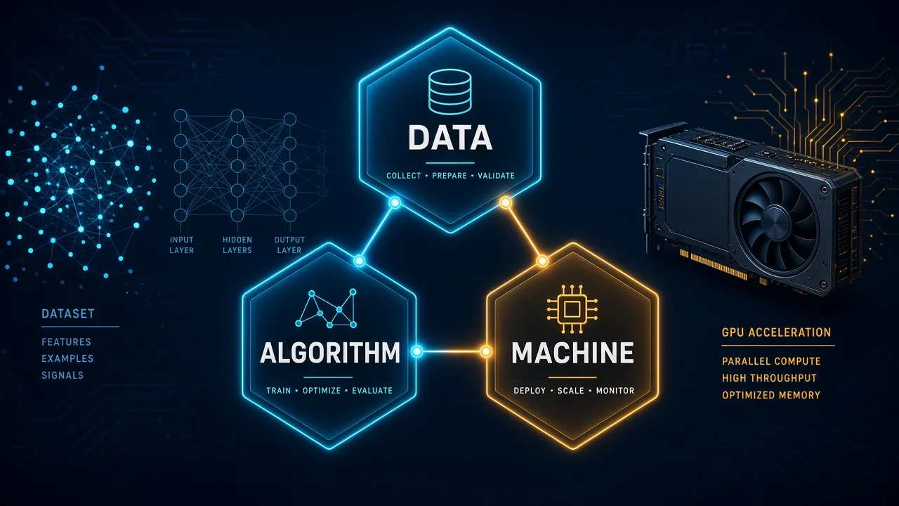
Table Of Content
- 1. The Shift: From Traditional ML to Applied ML
- 2. A Model Is Not a Complete System
- 3. Why Not Just Buy a Faster GPU?
- 4. The D·A·M Taxonomy: Data, Algorithm, and Machine
- 5. The Iron Law: Understanding Where Execution Time Goes
- 6. The Roofline Model: Is Your Workload Compute-Bound or Memory-Bound?
- 7. Model Compression: Making Models More Efficient
- 8. The Return on Compute: Is the Improvement Worth the Cost?
- 9. Bigger Models Are Not Always Better: The Chinchilla Insight
- 10. Putting Everything Together
- Conclusion: Think Beyond the Neural Network
Beyond Model Accuracy: Understanding Applied ML Through Data, Algorithms, and Hardware
Why building a better machine learning model is not always the same as building a better machine learning system.
1. The Shift: From Traditional ML to Applied ML
For a long time, the traditional view of Machine Learning has been relatively straightforward:
Dataset → Algorithm → Accuracy
We collect a dataset, select an algorithm, train a model, and evaluate its performance. If the model achieves 95% accuracy, we might consider it a successful experiment.
But there is a problem with this perspective: a model can perform exceptionally well in an experiment and still fail to solve the actual problem it was designed for.
Consider a hospital developing an ML model to predict whether patients are at risk of developing diabetes. Achieving 95% accuracy sounds impressive. However, what if the model takes several minutes to generate a prediction? What if it performs poorly on patients from a different demographic? Or what if its predictions never reach the doctors who need to make decisions?
The model might be technically successful, but the overall system is not necessarily useful.
This is where Applied Machine Learning introduces a different perspective:
Problem → Evidence → Decision → Impact
Let’s understand this progression:
- Problem: Identify a genuine real-world problem that needs to be solved.
- Evidence: Collect, process, and analyze relevant data to understand the problem.
- Decision: Use model predictions and other relevant information to support a decision.
- Impact: Measure whether the resulting decision actually improves the situation.
The important distinction is that Applied ML does not end when a model generates a prediction. It ends when that prediction contributes to a meaningful real-world outcome.
2. A Model Is Not a Complete System
One of the most important principles in Applied ML is:
Model ≠ Complete System
A machine learning model is only one component of a larger system.
Consider an ML-powered application that identifies fraudulent financial transactions.
The complete process might look like this:
- A transaction arrives.
- The system retrieves relevant customer and transaction information.
- Data preprocessing and feature extraction take place.
- The ML model generates a fraud probability.
- A decision engine determines whether to approve, reject, or flag the transaction.
- The result is delivered to the relevant system or user.
Notice that only one part of this entire process involves the actual ML model.
Other components include data retrieval, preprocessing, memory transfers, network communication, queue management, and decision-making.
Consequently, the overall performance of an ML application depends on much more than the model’s inference speed or accuracy.
This leads us to an important question:
If our ML application is slow, should we immediately buy a faster GPU?
Not necessarily.
3. Why Not Just Buy a Faster GPU?
Imagine we are developing an ML-powered application with a latency requirement of 30 milliseconds.
Our initial system has the following performance:
| Component | Execution time |
|---|---|
| Data preprocessing | 12 ms |
| Queue waiting | 8 ms |
| Data movement | 10 ms |
| Model inference | 10 ms |
| Total | 40 ms |
Our target is 30 ms, but the application takes 40 ms.
A common reaction would be to purchase a faster GPU.
Suppose the new GPU reduces model inference time from 10 ms to 7 ms.
The new performance becomes:
We have improved GPU inference performance by 30%, but the overall application latency has only improved from 40 ms to 37 ms.
We are still missing our 30 ms requirement.
Why?
Because the GPU was not the only bottleneck. Data preprocessing, queue waiting, and data movement also consume significant time.
This illustrates a fundamental principle of ML Systems Engineering:
First identify the actual bottleneck, then optimize the appropriate component.
A faster GPU cannot automatically solve inefficient data pipelines, memory bottlenecks, or excessive system overhead.
4. The D·A·M Taxonomy: Data, Algorithm, and Machine
To understand the complete ML system, we can use the D·A·M Taxonomy.
D·A·M represents three fundamental components:
- D — Data: The information used to train and operate the model.
- A — Algorithm: The mathematical logic and architecture responsible for learning and prediction.
- M — Machine: The physical hardware that executes the computation.
Think of these components as three interconnected parts of an engineering system.
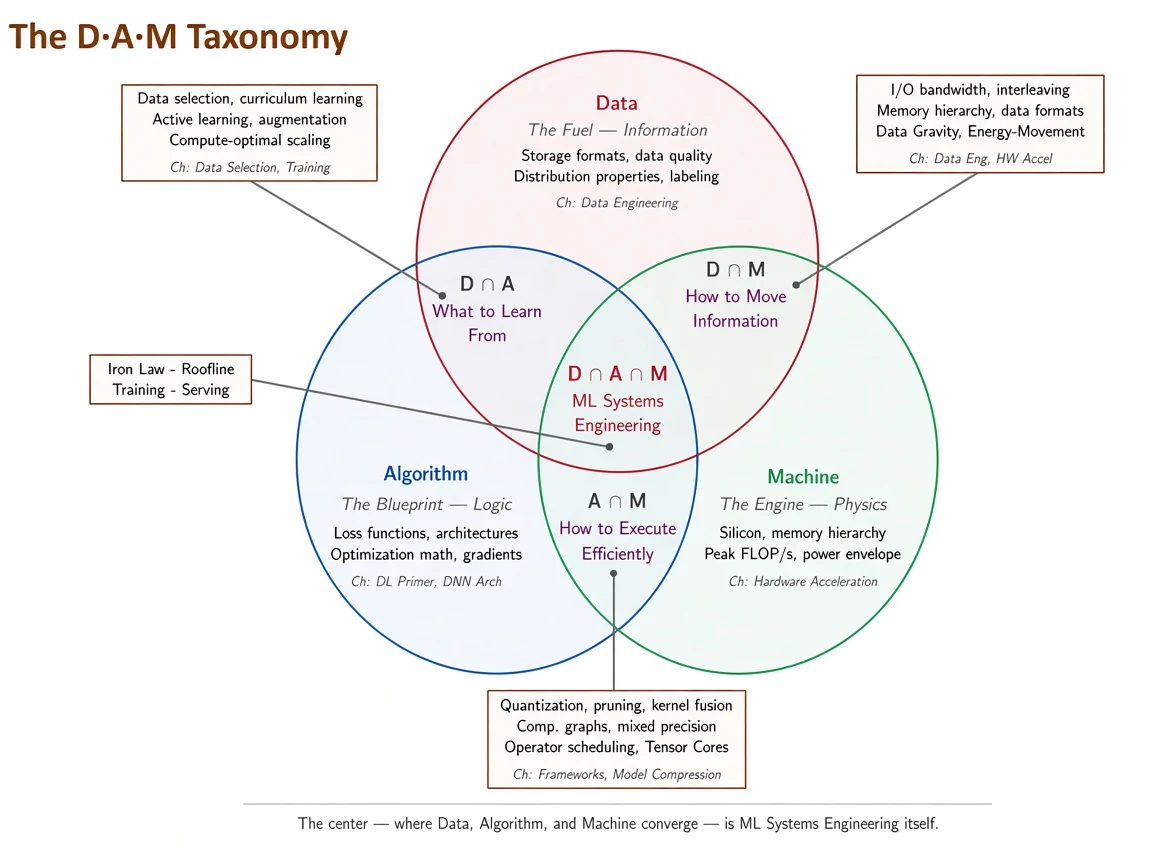
The center — where Data, Algorithm, and Machine converge — is ML Systems Engineering itself.
Data: The Fuel — Information
Data provides the information from which a machine learning model learns.
However, simply having more data does not guarantee better results.
Important considerations include:
- Data quality and labeling
- Data distribution
- Data selection
- Storage formats
- Data preprocessing
- Data movement
For example, suppose we have one million images for training an image classification model. If a significant portion of those images is incorrectly labeled, the model may learn incorrect patterns.
Therefore, selecting and preparing appropriate data can be more valuable than simply increasing dataset size.
Algorithm: The Blueprint — Logic
The algorithm defines how a model learns from data and generates predictions.
This includes:
- Neural network architectures
- Loss functions
- Optimization algorithms
- Gradients
- Training strategies
For example, a CNN, RNN, or Transformer can learn different types of patterns depending on its architecture and the problem being addressed.
The choice of algorithm affects not only prediction quality but also computational requirements.
Machine: The Engine — Physics
The machine represents the hardware responsible for executing ML computations.
This includes:
- CPUs and GPUs
- Memory hierarchy
- Processing throughput
- Memory bandwidth
- Power consumption
- Specialized accelerators such as Tensor Cores
Even a mathematically efficient algorithm can perform poorly if the hardware cannot execute it efficiently.
For example, a GPU might have enormous computational capacity but remain underutilized because data cannot be transferred into its memory quickly enough.
Why These Three Components Must Be Optimized Together
The most interesting part of the D·A·M Taxonomy is the intersection between these components.
Data ∩ Algorithm: What to Learn From
This intersection focuses on improving the learning process through better data and training strategies.
Examples include:
- Data selection
- Curriculum learning
- Active learning
- Data augmentation
- Compute-optimal scaling
Data ∩ Machine: How to Move Information
This intersection focuses on efficiently transferring information between storage, memory, and processors.
Examples include:
- I/O bandwidth
- Data prefetching
- Memory hierarchy
- Data formats
- Energy-efficient data movement
Algorithm ∩ Machine: How to Execute Efficiently
This intersection focuses on adapting algorithms to available hardware.
Examples include:
- Quantization
- Pruning
- Kernel fusion
- Mixed precision
- Computational graphs
- Operator scheduling
Finally, when Data, Algorithm, and Machine converge, we get ML Systems Engineering.
The goal is not simply to optimize one component independently, but to build a system in which all three work efficiently together.
5. The Iron Law: Understanding Where Execution Time Goes
Before optimizing an ML system, we need to understand where its execution time is being spent.
The Iron Law equation is:
In plain words:
Total time = time moving data + time doing calculations + fixed overhead
This is a simplified additive performance model, rather than a universal exact formula. In real systems, computation and data transfer can overlap, and queueing or network delays may need separate treatment. Still, it is an excellent way to reason about bottlenecks.
Data term
The data term is:
- = how much data needs to be moved
- = how fast the machine can move it
Example
Suppose:
Then:
So 400 ms is spent just moving data — like downloading a 40 MB file with a 100 MB/s connection.
Compute term
The compute term is:
- = how many calculations / operations are required
- = maximum calculation speed of the hardware
- = how much of that maximum performance you actually achieve (hardware utilization)
Example
- Maximum performance:
- Hardware utilization:
- Effective performance:
- Model requirement:
Then:
So 167 ms is spent actually computing the neural network.
Overhead term
covers costs that are not useful mathematical calculations, including:
- Scheduling
- Synchronization
- Launching GPU kernels
- Network communication
- Serialization
For the examples below, take:
Putting the terms together — data-bound example
Using the numbers above:
Breakdown:
- Data movement = 400 ms ← biggest
- Compute = 167 ms
- Overhead = 5 ms
Therefore this system is data-bound.
Buying a much faster GPU may not help much. You should first investigate ways of reducing data movement or increasing effective bandwidth.
Compute-bound example
Now consider a different system:
- Data =
- Compute = ← biggest
- Overhead =
Here the system is compute-bound.
Therefore, improving compute performance could make a significant difference.
The one thing to remember
The Iron Law is essentially asking:
“Where is my time actually going?”
- Data term is largest → Data-bound
- Compute term is largest → Compute-bound
- Overhead term is largest → Latency / overhead-bound
That is why optimizing the wrong component often produces disappointing results.
6. The Roofline Model: Is Your Workload Compute-Bound or Memory-Bound?
Another useful concept in ML Systems Engineering is the Roofline Model.
It helps us understand whether an application is limited by computational throughput or memory bandwidth.
Compute-bound workloads
A compute-bound workload spends most of its time performing mathematical operations.
Its performance is primarily limited by the processor’s computational capacity.
For example, a workload performing a large number of matrix multiplications may be compute-bound.
In this situation, improving GPU processing throughput can significantly improve performance.
Memory-bound workloads
A memory-bound workload spends a significant amount of time waiting for data to move between memory and processing units.
The GPU may have sufficient computational capacity, but it cannot receive data quickly enough to remain fully utilized.
In this situation, increasing computational throughput alone might not help much.
Improving memory bandwidth, reducing data transfers, or optimizing data access patterns may be more effective.
The Roofline Model uses the concept of arithmetic intensity:
A workload with high arithmetic intensity performs many operations for each byte transferred. It is more likely to be compute-bound.
A workload with low arithmetic intensity performs relatively few operations per byte transferred. It is more likely to be memory-bound.
This distinction helps engineers determine which hardware or software optimization is likely to provide the greatest benefit.
7. Model Compression: Making Models More Efficient
Once we understand the bottleneck, we can explore different optimization techniques.
Three particularly important techniques are knowledge distillation, pruning, and quantization.
Knowledge Distillation
Knowledge distillation involves training a smaller model (student) to reproduce useful behavior learned by a larger model (teacher).
For example:
- Teacher model: 12 Transformer layers
- Student model: 6 Transformer layers
Instead of training the smaller model only on original labels, we can use the teacher’s output probabilities to provide additional learning signals.
The student learns to approximate the teacher’s behavior while using fewer parameters and potentially requiring less computation.
The objective is to achieve a useful balance between model performance and computational cost.
Quantization
Neural networks frequently use floating-point numbers such as FP32 or FP16.
Quantization reduces the numerical precision used to represent model weights and sometimes activations.
For example:
FP16 → INT8
FP16 uses 16 bits per value, whereas INT8 uses 8 bits.
This can provide several benefits:
- Lower model memory requirements
- Reduced memory bandwidth consumption
- Faster computation on hardware supporting efficient INT8 operations
- Lower inference costs
For example, storing one billion values using FP16 requires approximately 2 GB of memory.
Using INT8 requires approximately 1 GB.
That is a 50% reduction in storage requirements for those values.
However, quantization can introduce numerical errors and potentially reduce model accuracy. Therefore, the resulting model must be evaluated carefully.
Pruning
Pruning removes parameters or structures that contribute relatively little to model performance.
The objective is to reduce model complexity and potentially improve execution efficiency.
However, removing weights does not automatically make a model faster. Actual speed improvements depend on the hardware and whether the resulting sparsity can be efficiently exploited.
8. The Return on Compute: Is the Improvement Worth the Cost?
Optimization is not free.
Reducing inference time, improving accuracy, or compressing a model may require additional engineering effort, computational resources, or trade-offs.
This raises another important question:
Is the improvement worth the additional computational cost?
One way to think about this is through Return on Compute (RoC):
This is a conceptual metric rather than a universal standard.
It represents how much additional model quality we obtain for additional computational investment.
For example:
| Experiment | Accuracy | Compute cost |
|---|---|---|
| Model A | 90% | 10 units |
| Model B | 93% | 20 units |
| Model C | 94% | 40 units |
Moving from A to B gives us a 3-percentage-point accuracy improvement for 10 additional compute units.
Moving from B to C gives only 1 additional percentage point for 20 additional compute units.
The marginal return is decreasing.
This suggests that continuously increasing model size and computational investment may not always be the most effective strategy.
In real applications, we should also consider latency, memory usage, energy consumption, financial cost, and the actual value of the improvement.
9. Bigger Models Are Not Always Better: The Chinchilla Insight
Gopher: bigger model → better performance
For a long time, a common assumption in deep learning was:
Bigger model → better performance
Models such as Gopher reflected that mindset: spend the compute budget primarily on making the neural network huge.
That encouraged researchers to keep increasing parameter counts.
But model size is only one part of the equation. Training data and the overall compute budget also matter.
Chinchilla challenged that idea
The comparison is:
| Gopher | Chinchilla | |
|---|---|---|
| Parameters | 280B | 70B |
| Training tokens | ~300B | ~1.4T |
| Model size | Huge | 4× smaller |
| Training data | Less | ~4.7× more |
So Chinchilla essentially said:
Instead of spending the compute budget primarily on making the model huge, use a smaller model and train it on substantially more data.
Despite having only 70B parameters, Chinchilla outperformed the much larger Gopher on many tasks while using roughly the same training-compute budget.
Largest model ≠ Best model
The important thing is the balance between model size, training data, and compute budget.
Under a fixed training-compute budget, model size and the number of training tokens should be scaled together. A smaller model trained on substantially more appropriate data can outperform a larger model that has been undertrained.
This changes how we think about model development.
Instead of asking:
“How can we make the model bigger?”
We should ask:
“Given our computational budget, what combination of model size and training data will produce the best result?”
This is another example of the D·A·M philosophy: optimize Data, Algorithm, and Machine together rather than focusing only on the neural network.
10. Putting Everything Together
Let’s imagine we are building an AI-powered application that needs to classify images within 30 milliseconds.
Our initial model is accurate but fails to meet the latency requirement.
Instead of immediately purchasing a more expensive GPU, we investigate the complete system.
Step 1: Identify the bottleneck
Measure preprocessing, data movement, queue waiting, and model inference separately.
Step 2: Analyze the hardware limitations
Determine whether the workload is compute-bound or memory-bound using performance profiling and Roofline-style analysis.
Step 3: Optimize the appropriate component
- If data movement is the problem, optimize memory access and data formats.
- If computation is the problem, investigate kernel optimization and hardware acceleration.
- If the model is unnecessarily large, consider distillation or pruning.
- If memory consumption is high, consider quantization.
Step 4: Evaluate the trade-offs
Measure accuracy, latency, memory consumption, energy usage, and computational cost.
Step 5: Measure real-world impact
Verify that the optimized system actually meets its requirements and improves the application.
This is the difference between simply optimizing a neural network and engineering a complete ML system.
Conclusion: Think Beyond the Neural Network
Applied Machine Learning requires a broader perspective than traditional model development.
A model’s accuracy is important, but it is only one dimension of success.
A practical ML system must consider:
- The quality and availability of data
- The efficiency of the learning algorithm
- The capabilities and limitations of hardware
- Data movement and computational bottlenecks
- Model performance versus computational cost
- The actual impact of predictions on real-world decisions
The D·A·M Taxonomy provides a useful mental model for understanding these relationships.
The Iron Law helps us reason about where execution time goes. The Roofline Model helps identify compute-bound and memory-bound workloads. Compression techniques help reduce computational requirements. Scaling research reminds us that bigger models are not automatically better.
Ultimately, the goal of Applied ML is not to build the biggest model, achieve the highest benchmark score, or purchase the fastest GPU.
It is to build the most effective system for solving the actual problem, within the available computational, financial, and operational constraints.
That is what separates building an ML model from engineering an ML system.