AI Search Algorithms: Comparison and Simulation

Table Of Content
- Cost Functions: How Do Search Algorithms Decide?
- The Game: OptimalTrek
- Comparing Search Strategies
- Problem Visualization
- Key Metrics for Comparison
- Algorithm Performance Comparison
- Quick Links
- Detailed Analysis with Visualizations
- Path Cost: What If Every Step Is Different?
- What if we combine both path cost and heuristic?
- Algorithm Selection Guide
- Best Practices for Implementation
- Final Thoughts
AI Search Algorithms: Comparison and Simulation
In this article, we'll compare a range of classic AI search algorithms: Breadth-First Search (BFS), Depth-First Search (DFS), Depth-Limited Search (DLS), Iterative Deepening Search (IDS), Uniform Cost Search (UCS), Greedy Best-First Search, A*, and Weighted A*. These algorithms are fundamental tools for solving pathfinding and search problems in artificial intelligence.
We can broadly classify these algorithms into two categories:
-
Uninformed (Blind) Search Algorithms:
These algorithms do not use any domain-specific knowledge (heuristics) about the goal's location.
Examples: BFS, DFS, DLS, IDS, UCS -
Informed (Heuristic) Search Algorithms:
These algorithms use heuristics to estimate the cost or distance to the goal, guiding the search more efficiently.
Examples: Greedy Best-First Search, A*, Weighted A*
Cost Functions: How Do Search Algorithms Decide?
A key concept in search algorithms is the cost function, which determines how each algorithm evaluates which node to explore next. Here are the main cost functions used:
-
Uninformed Search (BFS, DFS, DLS, IDS):
- These algorithms do not use a cost function or heuristic. They explore nodes based on order (queue, stack, or depth limit), not cost.
- For these:
- f(n) = depth(n) (for BFS/IDS) — nodes are explored in order of increasing depth (FIFO queue)
- f(n) = -depth(n) (for DFS) — nodes are explored in order of decreasing depth (LIFO stack)
- No explicit cost function for DLS/IDS, just depth limit
-
Uniform Cost Search (UCS):
- Explores nodes with the lowest path cost so far.
- g(n): Cost from start to node n
- f(n) = g(n)
- No heuristic is used.
-
Greedy Best-First Search:
- Explores nodes that appear closest to the goal, using only the heuristic.
- h(n): Estimated cost from node n to goal
- f(n) = h(n)
- Ignores path cost so far.
-
A* Search:
- Balances path cost so far and estimated cost to goal.
- g(n): Cost from start to node n
- h(n): Estimated cost from node n to goal
- f(n) = g(n) + h(n)
- Finds optimal paths if h(n) is admissible.
-
Weighted A* Search:
- Speeds up A* by weighting the heuristic.
- f(n) = g(n) + w × h(n), where w > 1
- May sacrifice optimality for speed.
Summary Table:
| Algorithm | Cost Function f(n) | Uses g(n)? | Uses h(n)? | Complete? | Optimal? |
|---|---|---|---|---|---|
| BFS | depth(n) | No | No | Yes | Yes |
| DFS | -depth(n) | No | No | Yes (finite space) | No |
| DLS/IDS | depth(n) (with limit) | No | No | DLS: No, IDS: Yes | DLS: No, IDS: Yes |
| UCS | g(n) | Yes | No | Yes | Yes |
| Best-First | h(n) | No | Yes | Yes | No |
| A* | g(n) + h(n) | Yes | Yes | Yes | Yes (if h admissible) |
| Weighted A* | g(n) + w × h(n) | Yes | Yes | Yes | Sometimes |
Where:
- g(n) = cost from start to node n
- h(n) = heuristic estimate from n to goal
- w = weight (w > 1 for Weighted A*)
These cost functions are at the heart of how each algorithm chooses its path through the search space.
The Game: OptimalTrek
Let's make these ideas concrete by introducing a simple grid-based game called OptimalTrek, where the player must move an object across a weighted grid to reach the goal in the lowest possible cost.
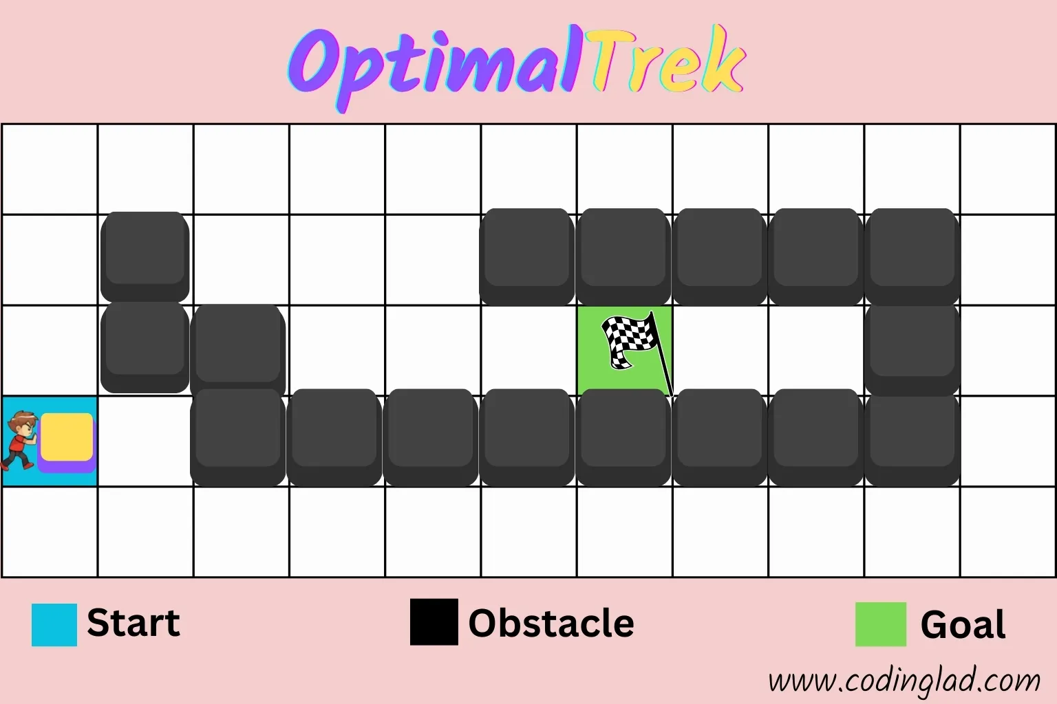
In this imagined game:
- The Start is marked in cyan (with your character)
- The Goal is the green flag
- Obstacles (black blocks) block your way
- You can only move up, down, left, or right—no diagonal moves allowed
These are the same rules that apply to many real-world pathfinding problems, from warehouse robots to delivery drones.
Movement Rules
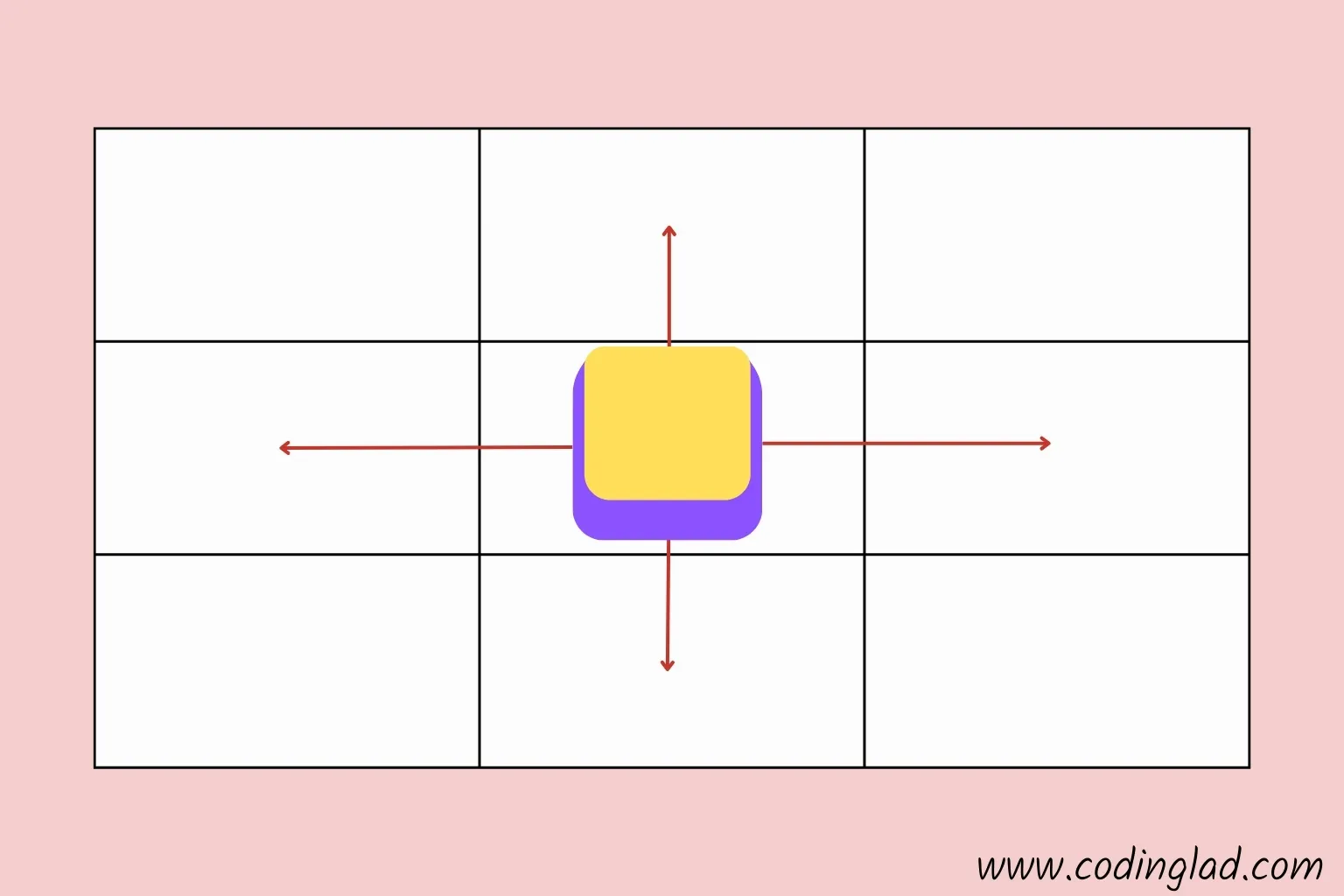
You can move one cell at a time, but you cannot pass through obstacles or move diagonally. The challenge is to find the best path to the goal!
Comparing Search Strategies
We'll use this grid world as a motivating example to compare different AI search algorithms. Each algorithm is a different strategy for solving the pathfinding problem:
- Some always find the shortest path (if one exists)
- Some use less memory
- Some are faster
- Some can handle different path costs
Let's see how each strategy performs in this world!
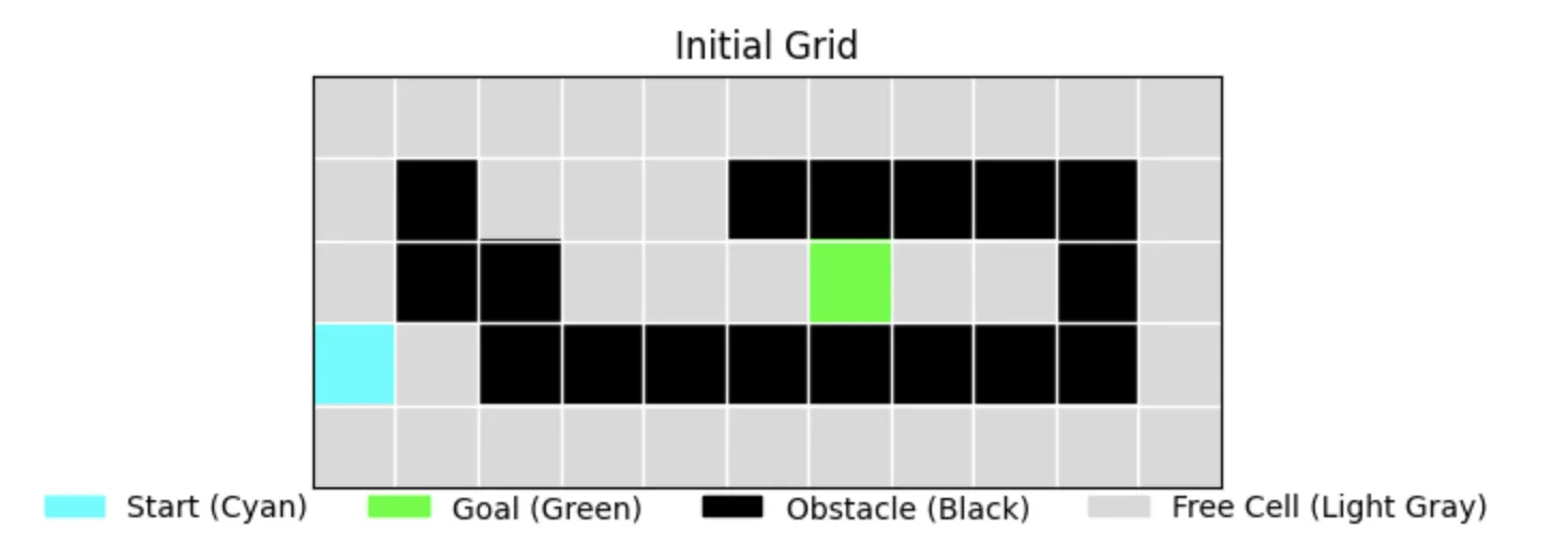
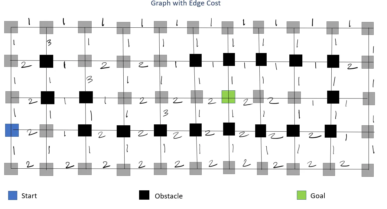
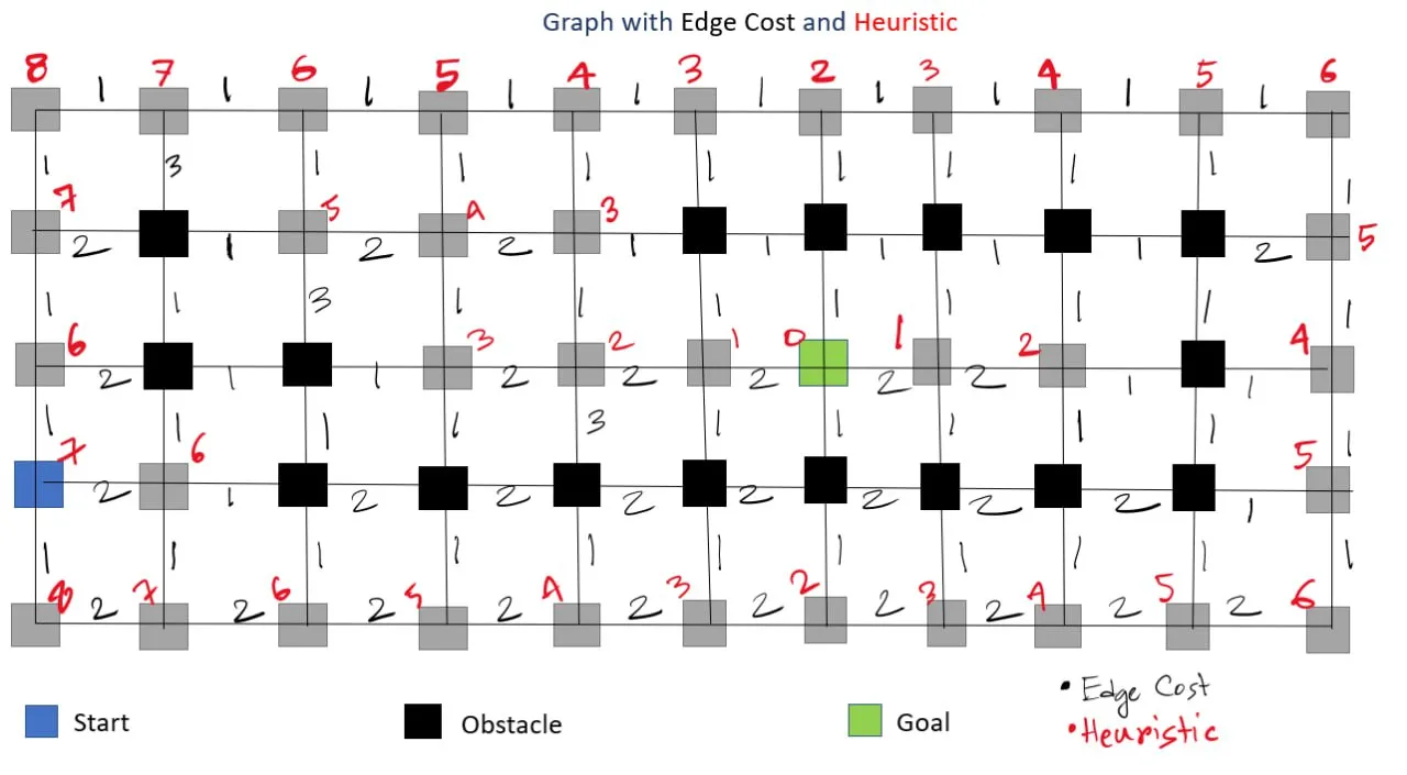
Problem Visualization
Let's start by looking at our test environment. We'll use a grid-based pathfinding problem to compare different search algorithms:
Key Metrics for Comparison
When evaluating search algorithms, we consider several critical metrics:
- Completeness: Does the algorithm guarantee finding a solution if one exists?
- Optimality: Does the algorithm find the optimal (best) solution?
- Memory Usage: How much memory does the algorithm require?
- Computational Time: How fast does the algorithm find a solution?
- Search Space: How efficiently does the algorithm explore the state space?
Algorithm Performance Comparison
Here's a detailed comparison of various search algorithms based on two runs of the same code with identical inputs, showing the consistency of our timing measurements:
First Run Results (Sorted by Time)
| Algorithm | Complete | Optimal | Time (s) | Nodes Stored | Nodes Expanded | Path Length |
|---|---|---|---|---|---|---|
| IDS | True | True | 0.000033 | 26 | 26 | 12 |
| DLS (limit=10) | False | False | 0.000039 | 26 | 26 | 0 |
| DFS | True | False | 0.000063 | 36 | 33 | 28 |
| Best-First | True | False | 0.000065 | 33 | 28 | 26 |
| BFS | True | True | 0.000068 | 32 | 30 | 12 |
| Weighted A* (w=2.0) | True | True | 0.000079 | 27 | 22 | 12 |
| A* | True | True | 0.000085 | 26 | 24 | 12 |
| UCS (Dijkstra) | True | True | 0.000106 | 30 | 28 | 12 |
Second Run Results (Sorted by Time)
| Algorithm | Complete | Optimal | Time (s) | Nodes Stored | Nodes Expanded | Path Length |
|---|---|---|---|---|---|---|
| IDS | True | True | 0.000032 | 26 | 26 | 12 |
| DLS (limit=10) | False | False | 0.000040 | 26 | 26 | 0 |
| Best-First | True | False | 0.000058 | 33 | 28 | 26 |
| DFS | True | False | 0.000063 | 36 | 33 | 28 |
| BFS | True | True | 0.000071 | 32 | 30 | 12 |
| Weighted A* (w=2.0) | True | True | 0.000078 | 27 | 22 | 12 |
| A* | True | True | 0.000087 | 26 | 24 | 12 |
| UCS (Dijkstra) | True | True | 0.000107 | 30 | 28 | 12 |
Key Observations
-
Timing Consistency:
- The timing measurements show good consistency between runs, with variations typically less than 0.00001s
- IDS consistently shows the fastest performance (0.000033s and 0.000032s)
- DLS shows very stable timing (0.000039s vs 0.000040s)
- All algorithms maintain their relative performance ordering between runs
-
Optimal Solutions:
- BFS, UCS, A*, Weighted A*, and IDS consistently find optimal paths (length 12)
- Best-First consistently finds suboptimal paths (length 26)
- DFS consistently finds suboptimal paths (length 28)
- DLS consistently fails to find a solution due to depth limit
-
Memory Usage:
- Memory usage (Nodes Stored) remains perfectly consistent across runs
- DFS consistently uses the most memory (36 nodes)
- A*, IDS, and DLS consistently use the least memory (26 nodes)
-
Path Length:
- Optimal path length (12) is consistently achieved by BFS, UCS, A*, Weighted A*, and IDS
- DFS consistently finds longer paths (28)
- Best-First consistently finds longer paths (26)
- DLS consistently fails to find a path (0)
-
Weighted A-star vs A-star Comparison:
- Weighted A* (w=2.0) is faster than A* (0.000079s vs 0.000085s in first run, 0.000078s vs 0.000087s in second run)
- Both algorithms find optimal paths (length 12)
- Weighted A* expands fewer nodes (22 vs 24)
- Weighted A* uses slightly more memory (27 vs 26 nodes stored)
- In this specific case, Weighted A* with w=2.0 provides a speed advantage while maintaining optimality
Quick Links
Feel free to experiment with different problem instances and parameters to see how the algorithms perform in your specific use case.
Open in Google Colab
Open in GitHub
All the code examples, visualizations, and comparison tests are available in a Google Colab notebook:
The notebook includes:
- Interactive implementations of all algorithms
- Visualization code for generating similar graphics
- Performance testing framework
- Additional test cases
- Customizable parameters
Detailed Analysis with Visualizations
1. Breadth-First Search (BFS)
The Reliable Workhorse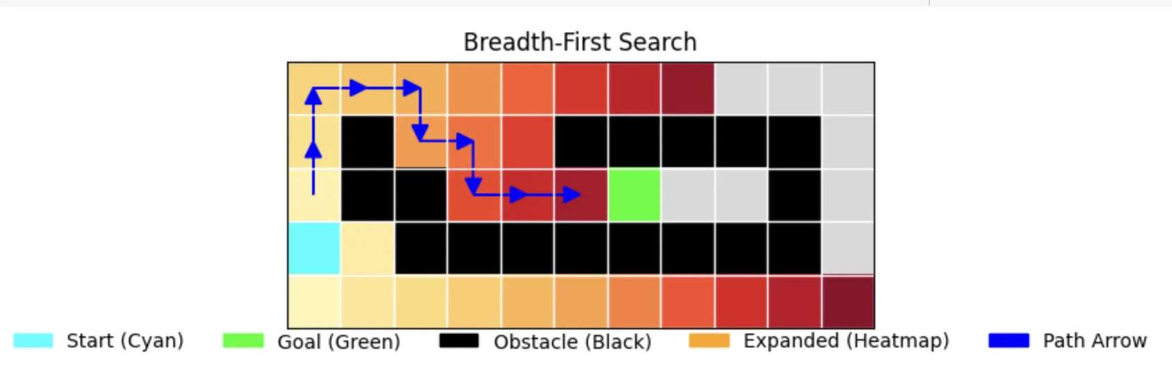
BFS explores the grid level by level, ensuring it finds the shortest path. As shown in the visualization:
- Yellow to red gradient shows the order of exploration
- Blue arrows indicate the final path
- Notice how it explores in concentric "waves" from the start position
function BFS(grid, start, goal):
    frontier = Queue()
    frontier.enqueue(start)
    came_from = {start: None}
    expanded = []

    while frontier is not empty:
        current = frontier.dequeue()
        expanded.append(current)

        if current == goal:
            return reconstruct_path(came_from, goal)

        for neighbor in get_neighbors(current):
            if neighbor not in came_from:
                came_from[neighbor] = current
                frontier.enqueue(neighbor)

return "No path found"Performance Characteristics:
- Time: 0.000068s (first run), 0.000071s (second run)
- Memory: 32 nodes stored
- Path Length: 12 (optimal)
- Nodes Expanded: 30
- Completeness: True
- Optimality: True
Simulation of BFS
2. Depth-First Search (DFS)
The Memory-Efficient Explorer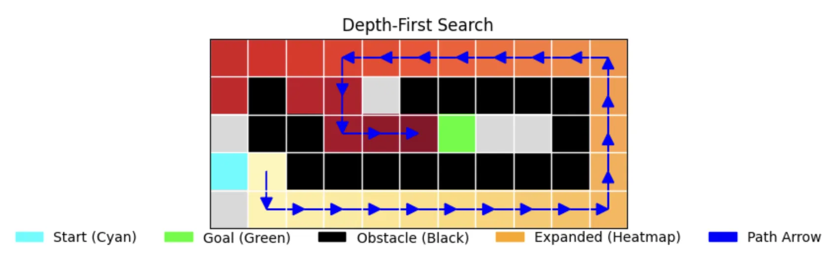
DFS dives deep into one path before backtracking. The visualization shows:
- A more linear exploration pattern
- Longer final path (28 steps vs BFS's 12)
- More efficient memory usage but suboptimal path
function DFS(grid, start, goal):
    frontier = Stack()
    frontier.push(start)
    came_from = {start: None}
    expanded = []

    while frontier is not empty:
        current = frontier.pop()

        if current in expanded:
            continue

        expanded.append(current)

        if current == goal:
            return reconstruct_path(came_from, goal)

        for neighbor in get_neighbors(current):
            if neighbor not in came_from:
                came_from[neighbor] = current
                frontier.push(neighbor)

return "No path found"Performance Characteristics:
- Time: 0.000063s (both runs)
- Memory: 36 nodes stored
- Path Length: 28 (non-optimal)
- Nodes Expanded: 33
- Completeness: True (in finite spaces with cycle handling)
- Optimality: False
Simulation of DFS
3. Depth-Limited Search (DLS)
The Bounded Explorer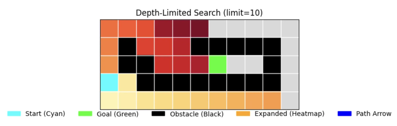
DLS with a limit of 10 shows:
- Limited exploration depth
- Incomplete search due to depth restriction
- Efficient memory usage but may miss solutions
function DLS(grid, start, goal, limit):
    came_from = {start: None}
    expanded = []

    function recursive_search(node, depth):
        expanded.append(node)

        if node == goal:
            return true

        if depth >= limit:
            return false

        for neighbor in get_neighbors(node):
            if neighbor not in came_from:
                came_from[neighbor] = node
                if recursive_search(neighbor, depth + 1):
                    return true

        return false

    found = recursive_search(start, 0)
    if found:
        return reconstruct_path(came_from, goal)
return "No path found within depth limit"Performance Characteristics:
- Time: 0.000039s (first run), 0.000040s (second run)
- Memory: 26 nodes stored
- Path Length: 0 (no solution found)
- Nodes Expanded: 26
- Completeness: False (due to depth limit)
- Optimality: False
Simulation of DLS
4. Iterative Deepening Search (IDS)
The Best of Both Worlds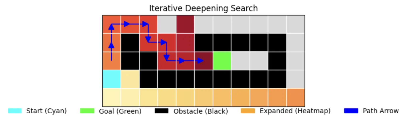
IDS combines the benefits of DFS and BFS:
- Gradually increases depth limit
- Complete like BFS
- Memory-efficient like DFS
- Shows excellent time performance (0.000033s and 0.000032s)
function IDS(grid, start, goal, max_limit):
    for limit from 0 to max_limit:
        result = DLS(grid, start, goal, limit)
        if result != "No path found within depth limit":
            return result
return "No path found"Performance Characteristics:
- Time: 0.000033s (first run), 0.000032s (second run)
- Memory: 26 nodes stored
- Path Length: 12 (optimal)
- Nodes Expanded: 26
- Completeness: True
- Optimality: True
Simulation of IDS
5. Best-First Search
The Eager Explorer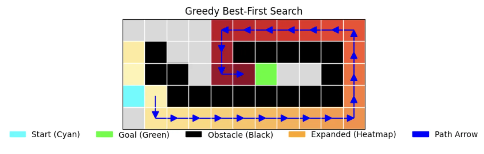
Best-First search uses heuristics to guide exploration:
- Focuses on promising directions
- May find suboptimal paths
- Efficient exploration but not guaranteed optimal
Manhattan Distance Heuristic
The Path Estimator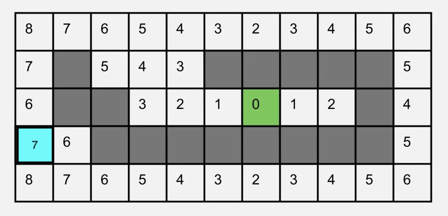
Manhattan distance, also known as city block distance, is named after the grid-like street layout of Manhattan, where you can only move along the streets (horizontally) and avenues (vertically), but not diagonally through buildings.
The Formula: To find the Manhattan distance between two points:
- Calculate the horizontal distance: subtract x-coordinates and take the absolute value
- Calculate the vertical distance: subtract y-coordinates and take the absolute value
- Add these two distances together
For example:
- If you're at point (2, 3) and want to reach point (5, 7):
- Horizontal distance = |5 - 2| = 3 blocks
- Vertical distance = |7 - 3| = 4 blocks
- Total Manhattan distance = 3 + 4 = 7 blocks
This method is perfect for grid-based pathfinding because:
- It matches how objects can move in a grid (no diagonal movement)
- It gives the exact minimum number of steps needed
- It's quick and simple to calculate
- It never underestimates the true distance
function manhattan_distance(a, b):
    return |a.x - b.x| + |a.y - b.y|
function heuristic(node, goal):
    return manhattan_distance(node, goal)
function BestFirst(grid, start, goal):
    frontier = PriorityQueue()
    frontier.push(start, heuristic(start, goal))
    came_from = {start: None}
    expanded = []

    while frontier is not empty:
        current = frontier.pop()
        expanded.append(current)

        if current == goal:
            return reconstruct_path(came_from, goal)

        for neighbor in get_neighbors(current):
            if neighbor not in came_from:
                came_from[neighbor] = current
                frontier.push(neighbor, heuristic(neighbor, goal))

return "No path found"Performance Characteristics:
- Time: 0.000065s (first run), 0.000058s (second run)
- Memory: 33 nodes stored
- Path Length: 26 (suboptimal)
- Nodes Expanded: 28
- Completeness: True
- Optimality: False
Simulation of Best-First Search
Path Cost: What If Every Step Is Different?
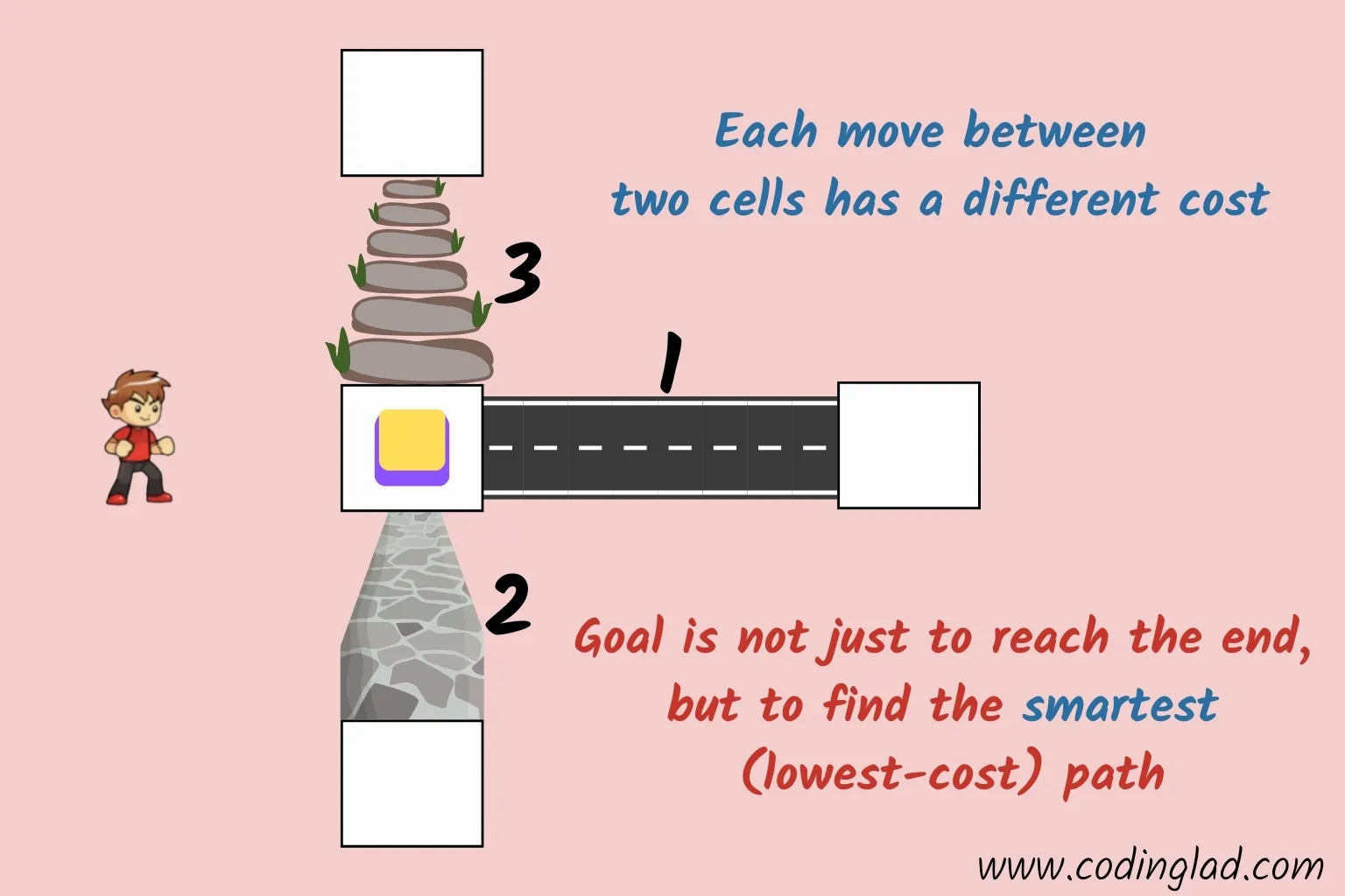
What if moving from one cell to another doesn't always cost the same? For example, moving through sand might cost more than moving on a road, or some paths might be longer or harder than others. In these cases, your goal isn't just to reach the finish, but to do so with the lowest total cost.
This is where advanced search strategies like Uniform Cost Search (UCS) and A* come into play, as they help you find the truly optimal path—even when costs vary.
6. Uniform Cost Search (UCS)
The Cost-Conscious Pathfinder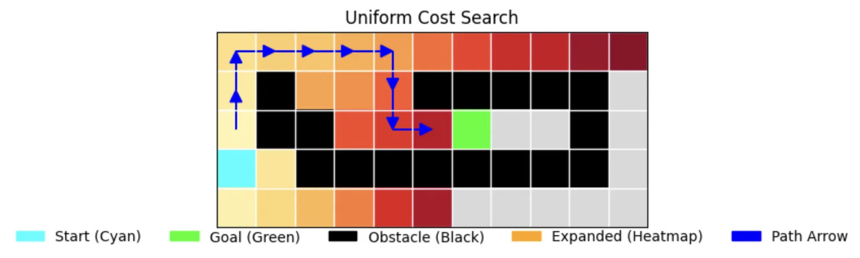
UCS (Dijkstra's algorithm) explores based on path cost:
- Guarantees optimal path
- Explores uniformly in all directions
- More computationally intensive (0.000106s and 0.000107s)
Performance Characteristics:
- Time: 0.000106s (first run), 0.000107s (second run)
- Memory: 30 nodes stored
- Path Length: 12 (optimal)
- Nodes Expanded: 28
- Completeness: True
- Optimality: True
function UCS(grid, start, goal):
    frontier = PriorityQueue()
    frontier.push(start, 0)
    came_from = {start: None}
    cost_so_far = {start: 0}
    expanded = []

    while frontier is not empty:
        current = frontier.pop()
        expanded.append(current)

        if current == goal:
            return reconstruct_path(came_from, goal)

        for neighbor, edge_cost in get_neighbors_with_cost(current):
            new_cost = cost_so_far[current] + edge_cost

            if neighbor not in cost_so_far or new_cost < cost_so_far[neighbor]:
                cost_so_far[neighbor] = new_cost
                came_from[neighbor] = current
                frontier.push(neighbor, new_cost)

return "No path found"Simulation of UCS
What if we combine both path cost and heuristic?
7. A* Search
The Optimal Pathfinder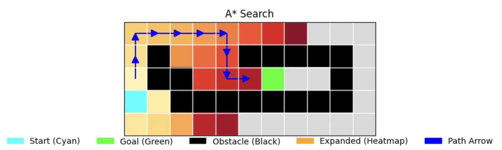
A* combines the benefits of UCS and Best-First Search:
- Uses both path cost and heuristic
- Guarantees optimal path when using admissible heuristics
- Efficient exploration (expands only 24 nodes)
- Balanced between speed and optimality
Performance Characteristics:
- Time: 0.000085s (first run), 0.000087s (second run)
- Memory: 26 nodes stored
- Path Length: 12 (optimal)
- Nodes Expanded: 24
- Completeness: True
- Optimality: True
function AStar(grid, start, goal):
    frontier = PriorityQueue()
    frontier.push(start, heuristic(start, goal))
    came_from = {start: None}
    g_score = {start: 0}
    expanded = []

    while frontier is not empty:
        current = frontier.pop()
        expanded.append(current)

        if current == goal:
            return reconstruct_path(came_from, goal)

        for neighbor, edge_cost in get_neighbors_with_cost(current):
            tentative_g = g_score[current] + edge_cost

            if neighbor not in g_score or tentative_g < g_score[neighbor]:
                came_from[neighbor] = current
                g_score[neighbor] = tentative_g
                f_score = tentative_g + heuristic(neighbor, goal)
                frontier.push(neighbor, f_score)

return "No path found"Simulation of A*
8. Weighted A* Search
The Speedy Compromise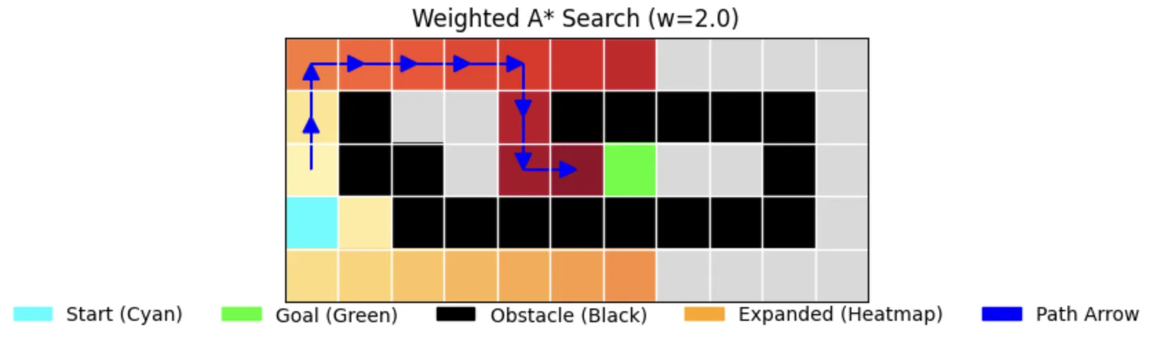
Weighted A* (w=2.0) trades optimality for speed:
- Uses weighted heuristic to bias towards goal
- Faster exploration (expands only 22 nodes)
- May find suboptimal paths
- Good balance between speed and path quality
Performance Characteristics:
- Time: 0.000079s (first run), 0.000078s (second run)
- Memory: 27 nodes stored
- Path Length: 12 (optimal in this case)
- Nodes Expanded: 22
- Completeness: True
- Optimality: True (in this specific case with w=2.0)
function WeightedAStar(grid, start, goal, weight):
    frontier = PriorityQueue()
    frontier.push(start, weight * heuristic(start, goal))
    came_from = {start: None}
    g_score = {start: 0}
    expanded = []

    while frontier is not empty:
        current = frontier.pop()
        expanded.append(current)

        if current == goal:
            return reconstruct_path(came_from, goal)

        for neighbor, edge_cost in get_neighbors_with_cost(current):
            tentative_g = g_score[current] + edge_cost

            if neighbor not in g_score or tentative_g < g_score[neighbor]:
                came_from[neighbor] = current
                g_score[neighbor] = tentative_g
                f_score = tentative_g + weight * heuristic(neighbor, goal)
                frontier.push(neighbor, f_score)

return "No path found"Simulation of Weighted A*
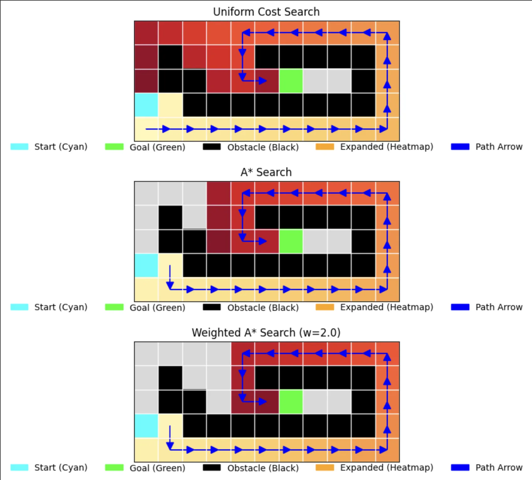
Manipulating Path: A Case Study
What happens if we increase the cost of a specific path segment, such as setting the cost of moving from (3,0) to (2,0) to 100? This effectively increases the cost of moving upward from the start cell(3.0), forcing the algorithm to consider alternative routes.
As expected, algorithms like BFS, DFS, DLS, IDS, and Greedy BFS remain unaffected since they are not cost-based and do not account for path costs. However, for cost-based algorithms like UCS, A*, and Weighted A*, the manipulation successfully alters the path. These algorithms adapt by choosing a longer but less costly path, moving downward instead of upward.
Algorithm Selection Guide
Based on our visualizations and metrics:
-
For Optimal Solutions:
- Use A* when you have a good heuristic
- Use BFS when memory isn't a concern
- Use UCS for weighted graphs
-
For Memory Efficiency:
- Use DFS or IDS when memory is limited
- Consider Weighted A* for a balance
-
For Speed:
- IDS shows the best time performance (0.000033s)
- Weighted A* offers good speed with reasonable memory usage
Best Practices for Implementation
-
Memory Management:
- Use efficient data structures
- Implement proper state pruning
- Consider iterative deepening for memory constraints
-
Performance Optimization:
- Choose appropriate heuristics
- Implement efficient state comparison
- Use priority queues for informed searches
-
Problem-Specific Considerations:
- Graph structure
- State space size
- Solution requirements
Final Thoughts
The visualizations clearly show how different algorithms explore the search space:
- BFS explores in waves, guaranteeing optimal paths
- DFS explores deeply, using less memory but finding longer paths
- UCS ensures optimal paths in weighted graphs
- Best-First balances exploration with heuristic guidance
Choose your algorithm based on:
- Need optimal solutions? Choose A* or BFS
- Memory constrained? Consider DFS or IDS
- Need speed? IDS or Weighted A* might be best
- Working with weights? UCS is your go-to
Remember that these results are from a specific test case. Always benchmark with your actual problem domain to make the best choice.